Saturday, 24 June 2017

Sprinkle Cookies | Recipe - ABC News

From the kitchen of Sprinkler System Installation Fort Worth Jeff Swartz

|


Servings:Over 8

Difficulty: Easy

Cook Time: 30-60 min

This fabulous recipe has been in Jeff Swartz's family for years and we're lucky he shared this with us! This recipe makes about 75 cookies, so it's the Sprinkler System Fort Worth perfect cookie to make for any holiday cookie swap.

Ingredients


For the cookie batter:

3 1/4 cup flour sifted

1 1/2 cup sugar

2 sticks butter or margarine

2 eggs

1/2 tsp. baking soda

1/2 tsp. baking powder

1 tsp. salt

1 tsp. almond extract

1 tbs. vanilla extract

1 cup sour cream

For the frosting:

1/2 box of confection sugar, (powdered sugar)

1/4 tsp. vanilla and almond extract

big tablespoon of marshmallow fluff

big tablespoon of spry (Crisco shortening)

add little bit of milk , to have the consistency of frosting

sprinkles

Cooking Directions

Makes 75 cookies.

Add sour cream, butter, and sugar together. Beat in both eggs and add almond and vanilla extracts.

In a separate bowl sift flour, baking soda, baking powder and salt. In another bowl beat both wet and dry ingredients together alternating between both. Let dough s it over night.

Preheat oven to 375. Using a teaspoon (or tablespoon depending on preferable size) spoon the batter onto an ungreased cookie sheet and bake for 5-10 minutes or until edges are slightly golden brown.

Be sure to cool cookies before frosting. In small http://cloverlawn.org/ mixing bowl beat Crisco, Fluff, sugar, and extracts. Splash in milk as needed to until mixture is smooth and has frosting consistency. Apply frosting and sprinkles and enjoy!

Recipe courtesy Jeff Swartz.

http://abcnews.go.com/GMA/recipe/sprinkle-cookies-15189555

Monday, 19 June 2017

Fire Sprinkler Recall - CBS News

About 35 million building sprinklers across the country need to be replaced because they might not work during fires, the government and the Pennsylvania manufacturer said Wednesday.

The sprinklers are installed in homes, offices, day-care facilities, hospitals and other buildings, the Consumer Product Safety Commission said.

Central Sprinkler Co., of Lansdale, Pa., discovered some of its sprinkler heads have O-ring seals that can corrode, said L. Dennis Kozlowski, chief executive of Tyco International Ltd., which owns the sprinkler company. The firm has received 13 reports of sprinklers failing to work during fires.

"We immediately shared our concerns with the authorities," Kozlowski told reporters. He noted the deterioration of the sprinklers "takes place over a very long period of time."


Tyco will provide free replacements for all the recalled sprinklers, the safety commission said. The first sprinklers replaced will be the oldest, those showing signs of damage or those in buildings such as nursing homes and hospitals.

The recall includes another 167,000 sprinklers sold by Gem Sprinkler Co. and Star Sprinkler Inc., which are also owned by Tyco, the safety commission said.

The recalled fire sprinkler heads have the words "CENTRAL" or "STAR", the letters "CSC", the letter "G" in a triangle, or a star-shaped symbol stamped on either the metal frame or the flower-shaped metal piece at one end of the sprinkler head.

About 2.5 million sprinklers installed in other countries, most of them in Cana da, are also included Sprinkler System Installation Richardson in the recall, said Central Sprinkler spokeswoman Anne Buchanan.

People seeking more information about how to replace their sprinklers should call the company toll-free at 1-800-871-3492.

Building owners, however, shouldn't shut off their sprinkler https://www.landscapingnetwork.com/ systems because of this recall, said Joseph Hirschmugl, a spokesman for Chicago-based Underwriters Laboratories (UL), which provides safety certifications and has been testing the recalled sprinklers.

"People should remember that sprinklers are important life saving devices," he said, noting that the recall is a precaution.

The vast majority of the recalled sprinklers are of the GB or glass-bulb type that contain alcohol or another liquid in a bulb mounted on the sprinkler head. Heat rising from a fire exp ands the liquid, causing the glass to shatter. That releases the sprinkler's plug and allows water onto the fire. An O-ring seal keeps the plug from leaking.

The testing organization said in April that some glass-bulb sprinklers produced by Central Sprinkler had crystallized deposits or corrosion around the rubber seal, which indicated leaking water.

It has recommended that the sprinklers be replaced since March 2000, but at the time, Brad McGee, a Tyco senior vice president, said it was too early to consider a recall or replacement of the sprinklers.


In 1998, Central Sprinkler recalled 8.4 million Omega brand fire sprinklers because thy could Sprinkler System fail in a fire. Those sprinklers, which were installed nationwide in schools, hospitals, hotels, offices and h omes, failed to activate in about 20 fires during the 1990s, causing injuries and millions of dollars in property damage, the safety commission said at the time.

MMI The Associated Press. All Rights Reserved. This material may not be published, broadcast, rewritten, or redistributed

http://www.cbsnews.com/news/fire-sprinkler-recall/

Saturday, 17 June 2017

Landscape

From Wikipedia, the free encyclopedia

For other uses, see Landscape (disambiguation).

A landscape is the visible features of an area of land, its landforms and how they integrate with natural or man-made features.[1]


A prairie: Badlands National Park, South Dakota, USA.


Tropical rainforest, Fatu Hiva Island, Marquesas Islands, French Polynesia.


Tundra in Siberia, Russia.


Taiga (Boreal forest), Alaska, US.


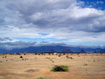
A desert: The rainshadow region of Tirunelveli, India.


A wetland: Viru Bog in Lahemaa National Park in Estonia.


Th e Aletsch Glacier, the largest glacier in the Swiss Alps.


Large fields of modern farmland, Dorset, England

A landscape includes the physical elements of geophysically defined landforms such as (ice-capped) mountains, hills, water bodies such as rivers, lakes, ponds and the sea, living elements of land cover including indigenous vegetation, human elements including different forms of land use, buildings and structures, and transitory elements such as lighting and weather conditions.

Com bining both their physical origins and the cultural overlay of human presence, often created over millennia, landscapes reflect a living synthesis of people and place that is vital to local and national identity. The character of a landscape helps define the self-image of the people who inhabit it and a sense of place that differentiates one region from other regions. It is the dynamic backdrop to people's lives. Landscape can be as varied as farmland, a landscape park, or wilderness.

The earth has a vast range of landscapes, including the icy landscapes of polar regions, mountainous landscapes, vast arid desert landscapes, islands and coastal landscapes, densely forested or wooded landscapes including past boreal forests and tropical rainforests, and agricultural landscapes of temperate and tropical regions.

The activity of modifying the visible features of an area of land is referred to as landscaping.

Contents

1 Definition and etymology

2 Physic al landscape

2.1 Geomorphology: The physical evolution of landscape

2.1.1 List of different types of landscape

2.2 Landscape ecology

2.3 Integrated landscape management

2.4 Landscape archaeology

2.5 Cultural landscape

3 Human conceptions and representations of landscape

3.1 Landscape gardens

3.2 Landscape architecture

3.3 Landscape and literature

3.3.1 The earliest landscape literature

3.3.2 Topographical poetry

3.3.3 The Romantic era in Britain

3.3.4 Europe

3.3.5 North America

3.4 Asia

3.4.1 China

3.5 Landscape art

3.5.1 Landscape photography

3.5.2 Landscape painting

4 Gallery of landscape paintings from different periods

5 See also

6 References

7 External links

Definition and etymology


Autumn landscape in Rybiniszki, Latvia, watercolor by Stanis?aw Mas?owski, 1902 (National Museum in Warsaw, Poland)

There are several definitions of what constitutes a landscape, depending on context. In common usage however, a landscape refers either to all the visible features of an area of land (usually rural), often considered in terms of aesthetic appeal, or to a pictorial representation of an area of countryside, specifically within the genre of landscape painting. When people deliberately improve the aesthetic appearance of a piece of land--by changing contours and vegetation, etc.--it is said to have been landscaped,[1] though the result may not constitute a landscape according to some definitions.

The word landscape (landscipe or landscaef) arrived in England--and therefore into the English language--after the fifth century, following the arrival of the Anglo-Saxons; these terms referred to a system of human-made spaces on the land. The term landscape emerged around the turn of the sixteenth century to denote a painting whose primary subject matter was natural scenery.[2]Land (a word from Germanic origin) may be taken in its sense of something to which people belong (as in England being the land of the English).[3] The suffix -scape is equivalent to the more common English suffix -ship.[3] The roots of -ship are etymologically akin to Old English sceppan or scyppan, meaning to shape. The suffix -schaft is related to the verb schaffen, so that -ship and shape are also etymologically linked. The modern form of the word, with its connotations of scenery, appeared in the late sixteenth century when the term landschap was introduced by Dutch painters who used it to refer to paintings of inland natural or rural scenery. The word landscape, first recorded in 1598, was borrowed from a Dutch painters' term.[4] The popular conception of the landscape that is reflected in dictionaries conveys both a particular and a general meaning, the particular referring to an area of the Earth's surface and the general being that which can be seen by an observer. An example of this second usage can be found as early as 1662 in the Book of Common Prayer:

Could we but climb where Moses stood,

And view the landscape over.

(General Hymns, verse 536).[5]

There are several words that are frequently associated with the word landscape:

Scenery: The natural features of a landscape considered in terms of their appearance, esp. when picturesque: spectacular views of mountain scenery.[1]

Setting: In works of narrative (especially fictional), it includes the historical moment in time and geographic location in which a story takes place, and helps initiate the main backdrop and mood for a story.[6]

Picturesque: The word literally means "in the manner of a picture; fit to be made into a picture", and used as early as 1703 (Oxford English Dictionary), and derived from an Italian term pittoresco, "in the manner of a painter". Gilpin's Essay on Prints (1768) defined picturesque as "a term expressive of that peculiar kind of beauty, which is agreeable in a picture" (p. xii).

A view: "A sight or prospect of some landscape or extended scene; an extent or area covered by the eye from one point" (OED).

Wilderness: An uncultivated, uninhabited, and inhospitable region.[1] See also Natural landscape.

Cityscape (also townscape): The urban equivalent of a landscape. In the visual arts a cityscape (urban landscape) is an artistic representation, such as a painting, drawing, print or photograph, of the physical aspects of a city or urban area.

Seascape: A photograph, painting, or other work of art which depicts the sea, in other words an example of marine art.

Physical landscape

Geomorphology: The physical evolution of landscape

Geomorphology is the scientific study of the origin and evolution of topographic and bathymetric features created by physical or chemical processes operating at or near Earth's surface. Geomorphologists seek to understand why landscapes look the way they do, to understand landform history and dynamics and to predict changes through a combination of field observations, physical ex periments and numerical modeling. Geomorphology is practiced within physical geography, geology, geodesy, engineering geology, archaeology and geotechnical engineering. This broad base of interests contributes to many research styles and interests within the field.[7]

The surface of Earth is modified by a combination of surface processes that sculpt landscapes, and geologic processes that cause tectonic uplift and subsidence, and shape the coastal geography. Surface processes comprise the action of water, wind, ice, fire, and living things on the surface of the Earth, along with chemical reactions that form soils and alter material properties, the stability and rate of change of topography under the force of gravity, and other factors, such as (in the very recent past) human alteration of the landscape. Many of these factors are strongly mediated by climate. Geologic processes include the uplift of mountain ranges, the growth of volcanoes, isostatic changes in land surface el evation (sometimes in response to surface processes), and the formation of deep sedimentary basins where the surface of Earth drops and is filled with material eroded from other parts of the landscape. The Earth surface and its topography therefore are an intersection of climatic, hydrologic, and biologic action with geologic processes.

List of different types of landscape

Desert, Plain, Taiga, Tundra, Wetland, Mountain, Mountain range, Cliff, Coast, Littoral zone, Glacier, Polar regions of Earth, Shrubland, Forest, Rainforest, Woodland, Jungle, Moors.


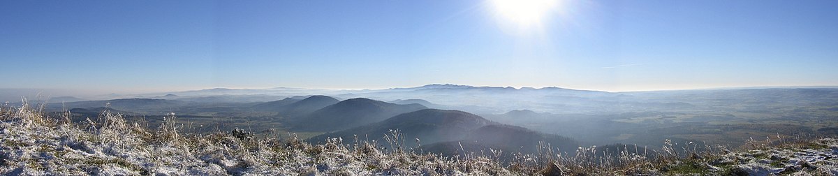
Panorama of the Chane des Puys from Puy de Dme in winter. Massif Central, France. An example of how past volcanic activity shaped a landscape

Landscape ecology

Landscape ecology is the science of studying and improving relationships between ecological processes in the environment and particular ecosystems. This is done within a variety of landscape scales, development spatial patterns, and organizational levels of research and policy.[8][9][10]

Landscape is a central concept in landscape ecology. It is, however, defined in quite different ways. For example:[11]Carl Troll conceives of landscape not as a mental construct but as an objectively given 'organic entity', a ''harmonic individuum of space''.[12]Ernst Neef[13] defines landscapes as sections within the uninterrupted earth-wide interconnec tion of geofactors which are defined as such on the basis of their uniformity in terms of a specific land use, and are thus defined in an anthropocentric and relativistic way.

According to Richard Forman and Michael Godron,[14] a landscape is a heterogeneous land area composed of a cluster of interacting ecosystems that is repeated in similar form throughout, whereby they list woods, meadows, marshes and villages as examples of a landscape's ecosystems, and state that a landscape is an area at least a few kilometres wide. John A. Wiens[15] opposes the traditional view expounded by Carl Troll, Isaak S. Zonneveld, Zev Naveh, Richard T. T. Forman/Michel Godron and others that landscapes are arenas in which humans interact with their environments on a kilometre-wide scale; instead, he defines 'landscape'--regardless of scale--as "the template on which spatial patterns influence ecological processes".[16] Some define 'landscape' as an area containing two or more ecosystems in clos e proximity.[17]

Integrated landscape management

Integrated landscape management is a way of managing a landscape that brings together multiple stakeholders, who collaborate to integrate policy and practice for their different land use objectives, with the purpose of achieving sustainable landscapes.[18][19] It recognises that, for example, one river basin can supply water for towns and agriculture, timber and food crops for smallholders and industry, and habitat for biodiversity; the way in which each one of these sectors pursues its goals can have impacts on the others. The intention is to minimise conflict between these different land use objectives and ecosystem services.[19] This approach draws on landscape ecology, as well as many related fields that also seek to integrate different land uses and users, such as watershed management.[18]

Proponents of integrated landscape management argue that it is well-suited to address complex global challenges, such as those that are the focus of the Sustainable Development Goals.[20] Integrated landscape management is increasingly taken up at the national,[21][22] local[23] and international level, for example the UN Environment Programme states that "UNEP champions the landscape approach de facto as it embodies the main elements of integrated ecosystem management".

Landscape archaeology

Main articles: Landscape archaeology and Historical ecology


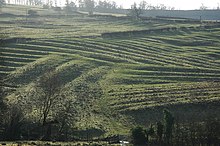
Medieval Ridge and Furrow above Wood Stanway, Gloucestershire, England.

Landscape archaeology or landscape history is the study of the way in which humanity has changed the physical appearance of the environment - both present and past. Landscape generally refers to both natural environments and environments constructed by human beings.[24]Natural landscapes are considered to be environments that have not been altered by humans in any shape or form.[25]Cultural landscapes, on the other hand, are environments that have been altered in some manner by people (including temporary structures and places, such as campsites, that are created by human beings).[26] Among archaeologists, the term landscape can refer to the meanings and alterations people mark onto their surroundings.[26][27] As such, landscape archaeology is often employed to study the human use of land over extensive periods of time.[27][28] Landscape archaeology can be summed up by Nicole Branton's statement:

"the landscapes in landscape archaeology may be as small as a single household or garden or as large as an empire", and "although resource exploitation, class, and power are frequent topics of landscape archaeology, landscape approaches are concerned with spatial, not necessarily ecological or economic, relationships. While similar to settlement archaeology and ecological archaeology, landscape approaches model places and spaces as dynamic participants in past behavior, not merely setting (affecting human action), or artifact (affected by human action)".[24]

Cultural landscape


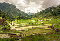
The Batad rice terraces, The Rice Terraces of the Philippine Cordilleras, the first site to be included in the UNESCO World Heritage List cultural landscape category in 1995.[29]

The concept of cultural landscapes can be found in the European tradition of landscape painting.[30] From the 16th century onwards, many European artists painted landscapes in favor of people, diminishing the people in their paintings to figures subsumed within broader, regionally specific landscapes.[31]

The geographer Otto Schlter is credited with having first formally used "cultural landscape" as an academic term in the early 20th century.[ 32] In 1908, Schlter argued that by defining geography as a Landschaftskunde (landscape science) this would give geography a logical subject matter shared by no other discipline.[32][33] He defined two forms of landscape: the Urlandschaft (transl. original landscape) or landscape that existed before major human induced changes and the Kulturlandschaft (transl. 'cultural landscape') a landscape created by human culture. The major task of geography was to trace the changes in these two landscapes.

It was Carl O. Sauer, a human geographer, who was probably the most influential in promoting and developing the idea of cultural landscapes.[34] Sauer was determined to stress the agency of culture as a force in shaping the visible features of the Earth's surface in delimited areas. Within his definition, the physical environment retains a central significance, as the medium with and through which human cultures act.[35] His classic definition of a 'cultural landscape' reads as follow s:

The cultural landscape is fashioned from a natural landscape by a cultural group. Culture is the agent, the natural area is the medium, the cultural landscape is the result.

A cultural landscape, as defined by the World Heritage Committee, is the "cultural properties [that] represent the combined works of nature and of man."[36]

The World Heritage Committee identifies three categories of cultural landscape, ranging from (i) those landscapes most deliberately 'shaped' by people, through (ii) full range of 'combined' works, to (iii) those least evidently 'shaped' by people (yet highly valued). The three categories extracted from the Committee's Operational Guidelines, are as follows:[37]

"A landscape designed and created intentionally by man";

an "organically evolved landscape" which may be a "relict (or fossil) landscape" or a "continuing landscape"; and

an "associative cultural landscape" which may be valued because of the "religious, art istic or cultural associations of the natural element".

Human conceptions and representations of landscape

Landscape gardens


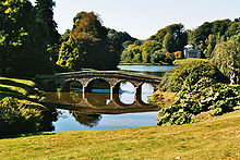
Stourhead garden, Wiltshire, England


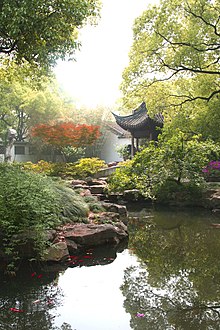
Jichang Garden in Wuxi (1506-1521)

See also: Landscaping, Landscape design, Landscape architecture, Garden, and Park

The Chinese garden is a landscape garden style which has evolved over three thousand years. It includes both the vast gardens of the Chinese emperors and members of the Imperial Family, built for pleasure and to impress, and the more intimate gardens created by scholars, poets, former government officials, soldiers and merchants, made for reflection and escape from the outside world. They create an idealized miniature landscape, which is meant to express the harmony that should exist between man and nature.[38] A typical Chinese garden is enclosed by walls and includes one or more ponds, scholar's rocks, trees and flowers, and an assortment of halls and pavilions within the garden, connected by winding paths and zig-zag galleries. By moving from structure to structure, visitors can view a series of carefully composed scenes, unrolling like a scroll of landscape paintings.[39]

The English landscape garden, also called English landscape park or simply the 'English garden', is a style of parkland garden intended to look as though it might be a natural landscape, although it may be very extensively re-arranged. It emerged in England in the early 18th century, and spread across Europe, replacing the more formal, symmetrical jardin la franaise of the 17th century as the principal style for large parks and gardens in Europe.[40] The English garden (and later French landscape garden) presented an idealized view of nature. It drew inspiration from paintings of landscapes by Claude Lorraine and Nicolas Poussin, and from the classic Chinese gardens of the East,[41] which had recently been described by European travellers and were realized in the Anglo-Chinese garden,[41] and the philosophy of Jean-Jacques Rousseau (1712 - 1778).

The English garden usually incl uded a lake, sweeps of gently rolling lawns set against groves of trees, and recreations of classical temples, Gothic ruins, bridges, and other picturesque architecture, designed to recreate an idyllic pastoral landscape. The work of Lancelot "Capability" Brown and Humphry Repton was particularly influential. By the end of the 18th century the English garden was being imitated by the French landscape garden, and as far away as St. Petersburg, Russia, in Pavlovsk, the gardens of the future Emperor Paul. It also had a major influence on the form of the public parks and gardens which appeared around the world in the 19th century.[42]

Landscape architecture


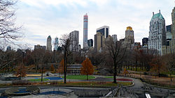
Central Park, New York City, US, designed by Frederick Law Olmsted.

Landscape architecture is a multi-disciplinary field, incorporating aspects of botany, horticulture, the fine arts, architecture, industrial design, geology and the earth sciences, environmental psychology, geography, and ecology. The activities of a landscape architect can range from the creation of public parks and parkways to site planning for campuses and corporate office parks, from the design of residential estates to the design of civil infrastructure and the management of large wilderness areas or reclamation of degraded landscapes such as mines or landfills. Lands cape architects work on all types of structures and external space- large or small, urban, suburban and rural, and with "hard" (built) and "soft" (planted) materials, while paying attention to ecological sustainability.

For the period before 1800, the history of landscape gardening (later called landscape architecture) is largely that of master planning and garden design for manor houses, palaces and royal properties, religious complexes, and centers of government. An example is the extensive work by Andr Le Ntre at Vaux-le-Vicomte and at the Palace of Versailles for King Louis XIV of France. The first person to write of making a landscape was Joseph Addison in 1712. The term landscape architecture was invented by Gilbert Laing Meason in 1828 and was first used as a professional title by Frederick Law Olmsted in 1863. During the latter 19th century, the term landscape architect became used by professional people who designed landscapes. Frederick Law Olmsted used the term 'la ndscape architecture' as a profession for the first time when designing Central Park, New York City, US. Here the combination of traditional landscape gardening and the emerging field of city planning gave landscape architecture its unique focus. This use of the term landscape architect became established after Frederick Law Olmsted, Jr. and others founded the American Society of Landscape Architects (ASLA) in 1899.

Landscape and literature

See also: Pastoral, British regional literature, and American literary regionalism

The earliest landscape literature


The Djabugay language group's mythical being, Damarri, transformed into a mountain range, is seen lying on his back above the Barron River Gorge, looking upwards to the skies, within north-east Australia's wet tropical forested landscape

Possibly the earliest landscape literature is found in Australian aboriginal myths (also known as Dreamtime or Dreaming stories, songlines, or Aboriginal oral literature), the stories traditionally performed by Aboriginal peoples[43] within each of the language groups across Australia. All such myths variously tell significant truths within each Aboriginal group's local landscape. They effectively layer the whole of the Australian continent's topography with cultural nuance and deeper meaning, and empower selected audiences with the accumulated wisdom and knowledge of Australian Aboriginal ancestors back to time immemorial.[44]

In the West pastoral poetry represent the earliest form of landscape literature, though this literary genre presents an idealized landscape peopled by shepherds and shepherdesses, and creates "an image of a peaceful uncorrupted existence; a kind of prelapsarian world".[45] The pastoral has its origins in the works of the Greek poet Theocritus (c. 316 - c. 260 BC). The Romantic period poet William Wordsworth created a modern, more realistic form of pastoral with Michael, A Pastoral Poem (1800).[46]

An early form of landscape poetry, Shanshui poetry, developed in China during the third and fourth centuries A.D.[47]


The Vale of Blackmore, the main setting for Thomas Hardy's novel Tess of the d'Urbervilles. Hambledon Hill towards Stourton Tower

Topographical poetry

Topographical poetry is a genre of poetry that describes, and often praises, a landscape or place. John Denham's 1642 poem "Cooper's Hill" established the genre, which peaked in popularity in 18th-century England. Examples of topographical verse date, however, to the Late Classical period, and can be found throughout the Medieval era and during the Renaissance. Though the earliest examples come mostly from continental Europe, the topographical poetry in the tradition originating with Denham concerns itself with the classics, and many of the various types of topographical verse, such as river, ruin, or hilltop poems were established by the early 17th century.[48]Alexander Pope's "Windsor Forest" (1713) a nd John Dyer's "Grongar Hill' (1762) are two other familiar examples. George Crabbe, the Suffolk regional poet, also wrote topographical poems, as did William Wordsworth, of which Lines written a few miles above Tintern Abbey is an obvious example.[49] More recently, Matthew Arnold's "The Scholar Gipsy" (1853) praises the Oxfordshire countryside, and W. H. Auden's "In Praise of Limestone" (1948) uses a limestone landscape as an allegory.[50]

Subgenres of topographical poetry include the country house poem, written in 17th-century England to compliment a wealthy patron, and the prospect poem, describing the view from a distance or a temporal view into the future, with the sense of opportunity or expectation. When understood broadly as landscape poetry and when assessed from its establishment to the present, topographical poetry can take on many formal situations and types of places. Kenneth Baker, in his "Introduction to The Faber Book of Landscape Poetry, identifies 37 variet ies and compiles poems from the 16th through the 20th centuries--from Edmund Spenser to Sylvia Plath--correspondent to each type, from "Walks and Surveys," to "Mountains, Hills, and the View from Above," to "Violation of Nature and the Landscape," to "Spirits and Ghosts."[51]

Common aesthetic registers of which topographical poetry makes use include pastoral imagery, the sublime, and the picturesque, which include images of rivers, ruins, moonlight, birdsong, and clouds, peasants, mountains, caves, and waterscapes.

Though describing a landscape or scenery, topographical poetry often, at least implicitly, addresses a political issue or the meaning of nationality in some way. The description of the landscape therefore becomes a poetic vehicle for a political message. For example, in John Denham's "Cooper's Hill," the speaker discusses the merits of the recently executed Charles I.[52]

The Romantic era in Britain

The Vision on Mount Snowdon

.......... .......................and on the shore

I found myself of a huge sea of mist,

Which meek and silent rested at my feet.

A hundred hills their dusky backs upheaved

All over this still ocean, and beyond,

Far, far beyond, the vapours shot themselves

In headlands, tongues, and promontory shapes, Into the sea, the real sea, that seemed

To dwindle and give up its majesty,

Usurped upon as far as sight could reach.

"

"

from The Prelude (1805), Book 13, lines 41-51.

by William Wordsworth

One important aspect of British Romanticism- evident in painting and literature as well as in politics and philosophy- was a change in the way people perceived and valued the landscape. In particular, after William Gilpin's Observations on the River Wye was published in 1770, the idea of the picturesque began to influence artists and viewers. Gilpin advocated approaching the landscape "by the rules of pi cturesque beauty,"[53] which emphasized contrast and variety. Edmund Burke's A Philosophical Enquiry into the Origin of Our Ideas of the Sublime and Beautiful (1757) was also an influential text, as was Longinus' On the Sublime (early A.D., Greece), which was translated into English from the French in 1739. From the 18th century, a taste for the sublime in the natural landscape emerged alongside the idea of the sublime in language; that is elevated rhetoric or speech.[54] A topographical poem that influenced the Romantics, was James Thomson's The Seasons (1726-30).[55] The changing landscape, brought about by the industrial and agricultural revolutions, with the expansion of the city and depopulation of the countryside, was another influences on the growth of the Romantic movement in Britain. The poor condition of workers, the new class conflicts, and the pollution of the environment all led to a reaction against urbanism and industrialisation and a new emphasis on the beauty and va lue of nature and landscape.[56] However, it was also a revolt against aristocratic social and political norms of the Age of Enlightenment, as well a reaction against the scientific rationalisation of nature.[57]

The poet William Wordsworth was a major contributor to the literature of landscape,[58] as was his contemporary poet and novelist Walter Scott. Scott's influence was felt throughout Europe, as well as on major Victorian novelists in Britain, such as Emily Bronte, Mrs Gaskell, George Eliot, and Thomas Hardy, as well as John Cowper Powys in the 20th-century.[59][60]Margaret Drabble in A Writer's Britain suggests that Thomas Hardy "is perhaps the greatest writer of rural life and landscape" in English.[61]

Europe

Among European writers http://www.ebay.com/sch/i.html?_nkw=lawn sprinkler influenced by Scott were Frenchmen Honor de Balzac and Alexandre Dumas and Italian Alessandro Manzoni.[62] M anzoni's famous novel The Betrothed was inspired by Walter Scott's Ivanhoe.[63]

North America

Also influenced by Romanticism's approach to landscape was the American novelist Fenimore Cooper, who was admired by Victor Hugo and Balzac and characterized as the "American Scott."[64]

Asia

China

Landscape in Chinese poetry has often been closely tied to Chinese landscape painting, which developed much earlier than in the West. Many poems evoke specific paintings, and some are written in more empty areas of the scroll itself. Many painters also wrote poetry, especially in the scholar-official or literati tradition. Landscape images were present in the early Shijing and the Chuci, but in later poetry the emphasis changed, as in painting]] to the Shan shui (Chinese: ?? lit. "mountain-water") style featuring wild mountains, rivers and lakes, rather than landscape as a setting for a human presence.[47]Shanshui poetry traditional Chinese: ???; simplified Chin ese: ??? developed in China during the third and fourth centuries AD[47] and left most of the varied landscapes of China largely unrepresented. Shan shui painting and poetry shows imaginary landscapes, though with features typical of some parts of South China; they remain popular to the present day.

Fields and Gardens poetry (simplified Chinese: ???; traditional Chinese: ???; pinyin: tinyun sh?; Wade-Giles: t'ien-yuan-shih; literally: "fields and gardens poetry"), in poetry) was a contrasting poetic movement which lasted for centuries, with a focused on the nature found in gardens, in backyards, and in the cultivated countryside. Fields and Gardens poetry is one of many Classical Chinese poetry genres. One of the main practitioners of the Fields and Gardens poetry genre was Tao Yuanming (also known as Tao Qian (365-427), among other names or versions of names).[65] Tao Yuanming has been regarded as the first great poet associated with the Fields and Gardens poetry genre.[66]< br>
Landscape art

Landscape photography

Main articles: Landscape photography, Conservation photography, and Aerial photography


The Tetons and the Snake River (1942) photograph by Ansel Adams

Many landscape photographs show little or no human activity and are created in the pursuit of a pure, unsullied depiction of nature[67] devoid of human influence, instead featuring subjects such as strongly define d landforms, weather, and ambient light. As with most forms of art, the definition of a landscape photograph is broad, and may include urban settings, industrial areas, and nature photography. Notable landscape photographers include Ansel Adams, Galen Rowell, Edward Weston, Ben Heine, Mark Gray and Fred Judge.

Landscape painting

Main articles: Landscape painting and Aerial landscape art


Salomon van Ruisdael, "View of Deventer" (1657).

The earlie st forms of art around the world depict little that could really be called landscape, although ground-lines and sometimes indications of mountains, trees or other natural features are included. The earliest "pure landscapes" with no human figures are frescos from Minoan Greece of around 1500 BCE.[68] Hunting scenes, especially those set in the enclosed vista of the reed beds of the Nile Delta from Ancient Egypt, can give a strong sense of place, but the emphasis is on individual plant forms and human and animal figures rather than the overall landscape setting. For a coherent depiction of a whole landscape, some rough system of perspective, or scaling for distance, is needed, and this seems from literary evidence to have first been developed in Ancient Greece in the Hellenistic period, although no large-scale examples survive. More ancient Roman landscapes survive, from the 1st century BCE onwards, especially frescos of landscapes decorating rooms that have been preserved at archaeo logical sites of Pompeii, Herculaneum and elsewhere, and mosaics.[69]

The Chinese ink painting tradition of shan shui ("mountain-water"), or "pure" landscape, in which the only sign of human life is usually a sage, or a glimpse of his hut, uses sophisticated landscape backgrounds to figure subjects, and landscape art of this period retains a classic and much-imitated status within the Chinese tradition.

Both the Roman and Chinese traditions typically show grand panoramas of imaginary landscapes, generally backed with a range of spectacular mountains - in China often with waterfalls and in Rome often including sea, lakes or rivers. These were frequently used to bridge the gap between a foreground scene with figures and a distant panoramic vista, a persistent problem for landscape artists.

A major contrast between landscape painting in the West and East Asia has been that while in the West until the 19th century it occupied a low position in the accepted hierarchy of genres, in East Asia the classic Chinese mountain-water ink painting was traditionally the most prestigious form of visual art. However, in the West, history painting came to require an extensive landscape background where appropriate, so the theory did not entirely work against the development of landscape painting - for several centuries landscapes were regularly promoted to the status of history painting by the addition of small figures to make a narrative scene, typically religious or mythological.

Dutch Golden Age painting of the 17th century saw the dramatic growth of landscape painting, in which many artists specialized, and the development of extremely subtle realist techniques for depicting light and weather. The popularity of landscapes in the Netherlands was in part a reflection of the virtual disappearance of religious painting in a Calvinist society, and the decline of religious painting in the 18th and 19th centuries all over Europe combined with Romanticism to give landscapes a much greater and more prestigious place in 19th-century art than they had assumed before.

In England, landscapes had initially been mostly backgrounds to portraits, typically suggesting the parks or estates of a landowner, though mostly painted in London by an artist who had never visited the site. the English tradition was founded by Anthony van Dyck and other, mostly Flemish, artists working in England. By the beginning of the 19th century the English artists with the highest modern reputations were mostly dedicated landscapists, showing the wide range of Romantic interpretations of the English landscape found in the works of John Constable, J.M.W. Turner and Samuel Palmer. However all these had difficulty establishing themselves in the contemporary art market, which still preferred history paintings and portraits.[70]


Thomas Cole "The Course of Empire The Arcadian or Pastoral State", US, 1836.

In Europe, as John Ruskin said,[71] and Sir Kenneth Clark confirmed, landscape painting was the "chief artistic creation of the nineteenth century", and "the dominant art", with the result that in the following period people were "apt to assume that the appreciation of natural beauty an d the painting of landscape is a normal and enduring part of our spiritual activity"[72]

The Romantic movement intensified the existing interest in landscape art, and remote and wild landscapes, which had been one recurring element in earlier landscape art, now became more prominent. The German Caspar David Friedrich had a distinctive style, influenced by his Danish training. To this he added a quasi-mystical Romanticism. French painters were slower to develop landscape painting, but from about the 1830s Jean-Baptiste-Camille Corot and other painters in the Barbizon School established a French landscape tradition that would become the most influential in Europe for a century, with the Impressionists and Post-Impressionists for the first time making landscape painting the main source of general stylistic innovation across all types of painting.

In the United States, the Hudson River School, prominent in the middle to late 19th century, is probably the best-known native development in landscape art. These painters created works of mammoth scale that attempted to capture the epic scope of the landscapes that inspired them. The work of Thomas Cole, the school's generally acknowledged founder, has much in common with the philosophical ideals of European landscape paintings -- a kind of secular faith in the spiritual benefits to be gained from the contemplation of natural beauty. Some of the later Hudson River School artists, such as Albert Bierstadt, created less comforting works that placed a greater emphasis (with a great deal of Romantic exaggeration) on the raw, even terrifying power of nature. The best examples of Canadian landscape art can be found in the works of the Group of Seven, prominent in the 1920s.[73]Emily Carr was also closely associated with the Group of Seven, though was never an official member. Although certainly less dominant in the period after World War I, many significant artists still painted landscapes in the wide variety of styles exemplified by Neil Welliver, Alex Katz, Milton Avery, Peter Doig, Andrew Wyeth, David Hockney and Sidney Nolan.

The term neo-romanticism is applied in British art history, to a loosely affiliated school of landscape painting that emerged around 1930 and continued until the early 1950s.[74] These painters looked back to 19th-century artists such as William Blake and Samuel Palmer, but were also influenced by French cubist and post-cubist artists such as Pablo Picasso, Andr Masson, and Pavel Tchelitchew (Clark and Clarke 2001; Hopkins 2001). This movement was motivated in part as a response to the threat of invasion during World War II. Artists particularly associated with the initiation of this movement included Paul Nash, John Piper, Henry Moore, Ivon Hitchens, and especially Graham Sutherland. A younger generation included John Minton, Michael Ayrton, John Craxton, Keith Vaughan, Robert Colquhoun, and Robert MacBryde (Button 1996).

Gallery of landscape painti ngs from different periods


Landscape with scene from the Odyssey, Rome, c. 60-40 BC.


Raphael, Madonna in the Meadow (1505 - 1506).


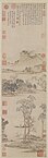
Spring in Kiangnan (1547) by Wen Cheng-Ming(1470-1559) (lower half detail).


Claude Lorrain, Landscape with Apollo Guarding the Herds of Admetus and Mercury stealing them (1645).


Albert Bierstadt, The Matterhorn (circa 1867).


Vincent van Gogh, Wheat Fields at Auvers Under Clouded Sky (1890).


Pablo Picasso, 1908, Paysage aux deux figures (Landscape with Two Figures)


Paul Nash, Wire (1918).


Carl Brandt: "reskutan, landscape",1921 (Sweden)


Emily Carr, Odds and Ends, 1939 (British Columbia, Canada)

See also

Australian aboriginal mythology, Mythologies of the indigenous peoples of the Americas, Aboriginal sacred site

Canal and Dam

Environmental health, Ecological health, Biodiversity, Landscape ecology, Pollution, and Erosion

Grand tour, Tourism, and Eco tourism

Hardscape, Urban design, and Urban park

Horticulture, Garden design, Japanese garden, Persian garden, List of landscape gardens, and Softscape

John Muir

Landscape mythology

Mining, Cornwall and West Devon Mining Landscape (This is a World Heritage site)
< br>Panorama

Sense of place

Nightscape

Taskscape

References

^ a b c d New Oxford American Dictionary

^ Olwig K.R., Recovering the Substantive Nature of Landscape, Annals of the A.A.G(1996),86,4,630-653

^ a b Olwig K.R., Representation and Alienation in the Political Landscape, cultural geographies (2005)12,19-40

^ Makhzoumi J. and Pungetti G., Ecological Landscape Design and Planning, Spon Routledge,(1999)

^ Found via Google Ngram

^ Obstfeld, 2002, p. 1, 65, 115, 171.

^ Summerfield, M.A., 1991, Global Geomorphology, Pearson Education Ltd, ISBN 0-582-30156-4.

^ Wu, J. 2006. Cross-disciplinarity, landscape ecology, and sustainability science. Landscape Ecology 21:1-4.

^ Wu, J. and R. Hobbs (Eds). 2007. Key Topics in Landscape Ecology. Cambridge University Press, Cambridge.

^ Wu, J. 2008. Landscape ecology. In: S. E. Jorgensen (ed), Encyclopedia of Ecology. Elsevier, Oxford.

^ Kirchh off, T., Trepl, L. and V. Vicenzotti, V. 2012: What is landscape ecology? An analysis and evaluation of six different conceptions. Landscape Research online first.

^ Troll, C. 2007: The geographic landscape and its investigation. In: Wiens, J.A., Moss, M.R., Turner, M.G. & Mladenoff, D.J. (eds): Foundation papers in landscape ecology. New York, Columbia University Press:71-101 [First published as: Troll, C. 1950: Die geographische Landschaft und ihre Erforschung. Studium Generale 3(4/5):163-181].

^ Neef, E. 1967: Die theoretischen Grundlagen der Landschaftslehre. Haack, Gotha; cf. Haase, G. and H. Richter 1983: Current trends in landscape research. GeoJournal 7(2):107-119.

^ Forman, R.T.T. and M. Godron, M. 1981: Patches and structural components for a landscape ecology. BioScience 31(10):733-740; Forman, R.T.T. and M. Godron 1986: Landscape ecology. Wiley, New York.

^ Wiens, J.A. and B.T. Milne, B.T. 1989: Scaling of 'landscapes' in landscape ecology, or , landscape ecology from the beetle's perspective. Landscape Ecology 3(2):87-96; Wiens, J.A.: The science and practice of landscape ecology. In: Klopatek, J.M. and R.H. Gardner (eds) 1999: Landscape ecological analyses: issues and applications. Springer, New York:371-383.

^ Wiens, J.A. 1999: The science and practice of landscape ecology. In: Klopatek, J.M. and R.H. Gardner (eds): Landscape ecological analyses: issues and applications. Springer, New York:371-383; cf. Wiens, J.A. 2005: Toward a unified landscape ecology. In: Wiens, J.A. and M.R. Moss (eds): Issues and perspectives in landscape ecology. Cambridge University Press, Cambridge:365-373.

^ Sanderson, J. and L. D. Harris (eds.). 2000. Landscape Ecology: A Top-Down Approach. Lewis Publishers, Boca Raton, Florida, USA.

^ a b Reed, J; Deakin, E; Sunderland, T (2015). "What are 'Integrated Landscape Approaches' and how effectively have they been implemented in the tropics: a systematic map protocol". Environ mental Evidence. 4:2. ISSN2047-2382.

^ a b Denier, L; Scherr, S; Shames, S; Chatterton, P; Hovani, L; Stam, N (2015). The Little Sustainable Landscapes Book. Oxford: Global Canopy Programme.

^ Landscapes for People Food and Nature (2015). "Integrated Landscape Management: The Means of Implementation for the Sustainable Development Goals" (PDF). Landscapes for People Food and Nature briefing.

^ "GMS Workshop on Landscape Approaches". Greater Mekong Subregion - Core Environment Program.

^ Republic of Indonesia. "Intended Nationally Determined Contribution" (PDF). UNFCCC submissions.

^ Landscapes for People Food and nature case studies http://peoplefoodandnature.org/analysis/all-publications/case-studies/

^ a b Branton, Nicole (2009) Landscape Approaches in Historical Archaeology: The Archaeology of Places. In International Handbook of Historic Archaeology, Majewski, Teresita and David Gaimster, eds. Springer:

^ Hood, Edward J. (1996) "S ocial Relations and the Cultural Landscape". In Landscape Archaeology:Reading and Interpreting the American Historical Landscape. Yamin, Rebecca and Karen Bescherer Metheny, eds. Knoxville:The University of Tennessee Press.

^ a b Spencer-Wood, Suzanne M. and Sherene Baugher. (2010) "Introduction to the Historical Archaeology of Powered Cultural Landscapes." International Journal of Historical Archaeology 14, pp. 463-474.

^ a b Gleason, Kathryn L. (1994). "To Bound and to Cultivate: An Introduction to the Archaeology of Gardens and Fields. In The Archaeology of Garden and Field. Miller, Naomi F. and Kathryn L. Gleason, eds. Philadelphia:University of Pennsylvania Press

^ Erika Martin Seibert. "Archaeology and Landscape", Accessed December 12, 2010.

^ Malig, Jojo (26 June 2012). "Philippine rice terraces no longer in danger". ABS-CBN News. Retrieved 26 June 2012.

^ PANNELL, S (2006) Reconciling Nature and Culture in a Global Context: Lessons form the World Heritage List. James Cook University. Cairns, Australia. Page 62

^ GIBSON, W.S (1989) Mirror of the Earth: The World Landscape in Sixteenth-Century Flemish Painting. Princeton University Press, Princeton, New Jersey

^ a b JAMES, P.E & MARTIN, G (1981) All Possible Worlds: A History of Geographical Ideas. John Wiley & Sons. New York, p.177.

^ ELKINS, T.H (1989) Human and Regional Geography in the German-speaking lands in the first forty years of the Twentieth Century. ENTRIKEN, J. Nicholas & BRUNN, Stanley D (Eds) Reflections on Richard Hartshorne's The nature of geography. Occasional publications of the Association of the American Geographers, Washington DC. Page 27

^ JAMES, P.E & MARTIN, G (1981) All Possible Worlds: A History of Geographical Ideas. John Wiley & Sons. New York. Page 321-324.

^ SAUER, C (1925) The Morphology of Landscape. University of California Publications in Geography. Number 22. Pages 19-53

^ UNESCO (2012) Operat ional Guidelines for the Implementation of the World Heritage Convention [1]. UNESCO World Heritage Centre. Paris. Page 14.

^ UNESCO (2005) Operational Guidelines for the Implementation of the World Heritage Convention. UNESCO World Heritage Centre. Paris. Page 84.

^ Michel Baridon, Les Jardins - paysagistes, jardiners, po?ts. p. 348

^ Records of the 21st conference of the UNESCO World Heritage Committee, describing Classical Chinese garden design and the gardens of Suzhou.

^ Yves-Marie Allain and Janine Christiany, L'Art des jardins en Europe, Citadelles and Mazenod, Paris, 2006.

^ a b Boults, Elizabeth and Chip Sullivan (2010). Illustrated History of Landscape Design. John Wiley and Sons. p.175. ISBN0-470-28933-3.

^ Lucia Impelluso, Jardins, potagers et labyrinthes, Mondatori Electra, Milan

^ Morris, C. (1994) "Oral Literature" in Horton, David (General Editor)

^ Morris, C. (1995) "An Approach to Ensure Continuity and Transmi ssion of the Rainforest Peoples' Oral Tradition", in Fourmile, H; Schnierer, S.; & Smith, A. (Eds) An Identification of Problems and Potential for Future Rainforest Aboriginal Cultural Survival and Self-Determination in the Wet Tropics. Centre for Aboriginal and Torres Strait Islander Participation Research and Development. Cairns, Australia

^ J. A. Cuddon, P. 644.

^ Peter V. Marinetti, Pastoral. London: Methuen, 1971, p.4.

^ a b c Yip, 130

^ Aubin, Robert Arnold. Topographical Poetry in XVIII-Century England. New York: The Modern Language Association of America, 1936, p. 3.

^ L. A. Cuddon, Dictionary of Literary Terms. London: Penguin, 1999,p.922

^ France, Alan W. (1990). "Gothic North and the Mezzogiorno in Auden's 'In Praise of Limestone'". Renascence. 42 (3): 141-148. doi:10.5840/renascence199042319.

^ Baker, Kenneth, ed. The Faber Book of Landscape Poetry. New York: Faber and Faber, 2000.

^ John Denham, "Cooper's Hill", (l l.111-119)

^ Gilpin, William, quoted in Baker, Kenneth, ed. The Faber Book of Landscape Poetry. New York: Faber and Faber, 2000, p. xxvi

^ In the late 17th century in England, John Dennis brought attention to Longinus' argument for the emotive power of figurative language in poetry.

^ Fulford, Tim. Landscape, LIberty, and Authority: Poetry, Criticism, and Politics from Thomson to Wordsworth. New York: Cambridge University Press, 1996., p.21'

^ Encyclopdia Britannica. "Romanticism". Retrieved 30 January 2008, from Encyclopdia Britannica Online. Britannica.com. Retrieved 24 August 2010.

^ Christopher Casey, (October 30, 2008). ""Grecian Grandeurs and the Rude Wasting of Old Time": Britain, the Elgin Marbles, and Post-Revolutionary Hellenism". Foundations. Volume III, Number 1. Retrieved 25 June 2009.

^ Margaret Drabble, A Writer's Britain (originally subtitled "Landscape in literature", 1979). New York: Thames & Hudson, 2000, p. 152.

^ "Walter Scott was the foremost literary figure of his days". Retrieved 2011-04-09.

^ Drabble,, p. 170

^ Drabble, p.91

^ Drabble,p. 166; "Alexandre Dumas": The official French site

^ From Georg Lukcs, "The Historical Novel" (1969): "In Italy Scott found a successor who, though in a single, isolated work, nevertheless broadened his tendencies with superb originality, in some respect surpassing him. We refer, of course, to Manzoni's I Promessi Sposi (The Betrothed). Scott himself recognized Manzoni's greatness. When in Milan Manzoni told him that he was his pupil, Scott replied that in that case Manzoni's was his best work. It is, however, very characteristic that while Scott was able to write a profusion of novels about English and Scottish society, Manzoni confined himself to this single masterpiece."

^ Phillips, 1913, p. 160

^ Yip, 163-169

^ Watson, 79

^ Mary Warner Marien (2006). Photography: A Cultural History. Laurence King Publishing. Page 136.

^ Honour & Fleming, 53. The only very complete example is now in the National Archaeological Museum, Athens

^ Honour & Fleming, 150-151

^ Reitlinger, 74-75, 85-87

^ Modern Painters, volume three, "Of the novelty of landscape".

^ Clark, 15-16.

^ "Landscapes" in Virtual Vault, an online exhibition of Canadian historical art at Library and Archives Canada

^ It was first labeled in March 1942 by the critic Raymond Mortimer in the New Statesman.

External links


Wikimedia Commons has media related to:
< br>landscapes (category)


Look up landscape in Wiktionary, the free dictionary.

Guardian podcasts: "Landscape and literature"

Authority control

GND: 4034343-1

BNF: cb11966944n (data)


Retrieved from "https://en.wikipedia.org/w/index.php?title=Landscape&oldid=778733963"

https://en.wikipedia.org/wiki/Landscape

Friday, 16 June 2017

Cooney & Conway Mesothelioma Attorneys

What Can Cooney & Conway's Mesothelioma Asbestos Attorney Help You With?

If you have seen the commercial on television for Best Attorney Cooney & Conway giving you a free Mesothelioma asbestos attorney consultation, you may wonder if you should really call to see what they can do for you. Cooney & Conway is an established law firm that has been in business since 1958. Whether you got mesothelioma through primary asbestos exposure or secondary asbestos exposure, it is in your benefit to see what Cooney & Conway can do for you. An asbestos attorney for mesothelioma cancer can help you find out whether your lung cancer, mesothelioma, rectal cancer, esophageal cancer, stomach or gastrointestinal cancer, intestinal cancer, asbestosis, pharyngeal and colon cancer is due asbestos exposure and help you get financial compensation for your pain and suffering.

Can Cooney & Conway Help Me Find Out How I Got Exposed To Mesoth elioma Cancer?

There are many ways you could have been exposed to mesothelioma through your profession or in the case of many women who have developed mesothelioma and other asbestos related diseases-through second hand contact with someone who was exposed to asbestos conditions. An asbestos attorney for mesothelioma cancer can help you find out how you got mesothelioma or other asbestos exposure related diseases and help you get the proper compensation.

You Could Have Been Affected By Asbestos Exposure Through The Following Ways

Mill and factory workers

Ship builders

Navy veterans

Plumbers

Electricians

Plasterers

Maintenance worker or Janitor

You could have also contracted mesothelioma through second hand exposure. If someone in the household was exposed to asbestos, someone who is living in the same household (women, children, younger and older adults, etc.,) could develop mesothelioma through second hand exposu re. An asbestos attorney for mesothelioma cancer can help you determine how you were exposed to asbestos and what Attorney College Station your legal options are.


The Cooney & Conway law firm says, says that they are experience mesothelioma cancer attorneys and they will work hard to hep you get get compensation for you and your family for your suffering. The number on the commercial is 800-3 22-5573 and they say they will give you a free consultation to determine if you are eligible for compensations.

How Can The Cooney & Conway law firm Help Me With My Asbestos Exposure Lawsuit?

As mesothelioma cancer lawyers, they have the resources that they need to find out whether there was negligence on the part or your employer or whomever exposed you to the deadly asbestos that caused your mesothelioma cancer. Their free consultaion will help you by asking pertinent questions so they know whether or not they can take your case. The consultation is free, so there is no risk on your part. Usually, mesothelioma cancer attorneys do not charge you anything until they get you compensation for your pain and suffering.

You should consult with more than one mesothelioma cancer attorney before you decide to go with one. If anyone is charging you any fees before they get you compensation, then they may not be working in your best interest and you may want to get other law firms to consider your case. It is really up to you who you deal with so you shouldn't have to feel bullied or pressured into making any decisions.

Take advantage of all the free consultations you can get, and then go with the firm you are most comfortable with.

Other law firm who promise you information from television commercials include:

Maune, Raichle, Hartley, French & Mudd Mesothelioma attorneys (800-500-9313)


A Note about Silver and Cancer. TheNational Instituteof Health(PubMed) has published documents about the effectiveness of silver in nano particles being used to treat affected cancer cells. There has been a lot of bad press about silver, but in truth the organized medical institutions still use it and used it widely and effectively before the invention of antibiotics. Before resigning yourself to death, speak to your doctor about trying all options, including so called "alternative." Consult a Natropath if you need to. There are ma ny writings about the use of silver helping to restore affected cancer cells to normal. Here is agood blog to read about the use of silver an cancer. Do your own study on pharmaceutical madecolloidal silverand how it can help you fight your disease. Always speak to your doctor about trying any new treatment including dietary supplements such as silver. Also, here's a good site that discusses the medical research of silver to treat serious diseases. I am not affiliated with theInviveorSilver Protein Mildwebsites nor the above blog, but they have some good information that could be useful to someone. Good Luck and just remember that thebible tells us, that for every illness, there is a treatment or cure.

Related Articles on Mesothelioma Cancers and Asbestos Related Diseases

Asbestos Exposure Symptoms: A List of Asbestos Lung Cancer Symptoms

Mesothelioma Cancer In Black Men

Asbestos Exposure From Shipyards, Papermills, etc-Contact Maine Mesothelioma Attorney

Cooney And Conway Mesothelioma Attorneys

Asbestos Help Now: Legal Help For Asbestos Exposure https://courtapps.in.gov/rollofattorneys Cancer

1-800-444-Meso

Mesothelioma Cancer Survival Story: Tom Harper

Facts About Mesothelioma

Best Books On Mesothelioma Cancer

http://www.infobarrel.com/Cooney__Conway_Mesothelioma_Attorneys

Artist Gives Famous Paintings Geeky Cartoon Makeovers

The classics meet Cartoon Network.

A Canadian artist who goes simply by Lothlenan created a Tumblr post that's been widely sharedduring the past week. The post features famous paintings reimagined with carefully chosen cartoon characters.


"Woman with a Parasol" by Claude Monet reimagined with Chu Totoro.

"I was doing a study of 'Mr. and Mrs. Andrews' by Thomas Gainsborough in my free time, trying to strengthen my painting skills," Lothlenan explained to HuffPost. "I was a little over halfway done when I decided I wanted to spice it up a little. I can't exactly say how the two threads joined in my head, but maybe it was because I'd recently seen some episodes of 'Adventure Time' with the Earl of Lemongrab and thought he'd sit quite well in the painting."


"Mr. and Mrs. Andrews" by Thomas Gainsborough reimagined with the Earl of Lemongrab and Lady Lemongrabs from "Adventure Time."

Lothlenan liked the way the painting came out and said that his friends got a kick out it. So, he decided to make it his thing.

"It became kind of like my amusing little twist. I strive to find subjects that resonate with the original painting," he said. "Sort of a personal challenge, but also something to make the process more entertaining."


"The Accolade" by Edmund Leighton reimagined with Link and Princess Zelda.

Lothlenan said he's always been into video games and manga. Some of his favorite cartoons include "Steven Universe," "Rick and Morty," "Adventure Time" and "absolutely anything by Studio Ghibli."

But he learned to appreci ate classic paintings when he was in college.


"The Swing" by Jean-Honor Fragonard reimagined with Rose Quartz from "Steven Universe."

"It wasn't until I hit university and had https://www.art.com/ an incredible professor that I developed a really strong appreciation for the old masters and their more modern successors," he said.


Lothlenan paints all of his pieces digitally and says that each of his cartoon recreations took about a week to make. The process is much more tedious than one might think.


"Portrait of Louis XIV" by Hyacinthe Rigaud reimagin ed with Ice King from "Adventure Time."

"As for the process itself, I always start with the backgrounds and, honestly, that's the most time-consuming part," Lothlenan told HuffPost. "It usually involves me trying to figure out how to approach the original artist's painting methods, and if there are specific brush techniques I need to account for to achieve a certain look."


"Self-portrait with Her Daughter" by lisabeth Loui se Vige Le Brun reimagined with Sailor Moon and Rini.

As for the popularity of these particular paintings, Lothlenan has a theory.


"Lovers on a Swing" by Pierre Auguste Cot reimagined withPrincess Bubblegum and Marceline from "Adventure Time."

"I think because it's two halves of the familiar, but in an unfamiliar way," he said.

He acknowledged fans might not instantly recognize the classic paintings that inspired him.

"I hope that my interpretations leave them walking away with a newfound appreciation for the original masterpiece," he added.

http://www.huffingtonpost.com/entry/artist-gives-famous-paintings-geeky-cartoon-makeovers-and-it-rules_us_5936c5b7e4b0cfcda917d634

Thursday, 15 June 2017

Get the Most Out Of Your Raised Bed Garden

Raised beds are a great way to create arable land just about anywhere. If you're looking to add a few extra square feet to your garden this summer, here are some great tips on how to get the most out of your raised beds.

Choosing the Right Spot

To get the most out of your raised beds, you need to choose the best spot. Look for a spot that gets at least six hours of full sun each day. Before building the beds, mark out your chosen spot with some stakes and string and then take a look throughout the day to ensure that all corners of the bed are getting regular and even sunlight. You also want to consider drainage. While not as important as sunlight, you will want to avoid putting you beds down in an area where water pools when it rains. For the best results, find a spot that sits on slightly higher ground than the rest of your yard.

Setting the Right Depth

A raised bed https://en.wikipedia.org/wiki/Landscap ing garden can be a great investment over time, but for those just starting out, the startup costs can be a little steep. To limit the amount of money that you spend on soil and lumber, you'll want to carefully consider how high to build the beds. For a basic vegetable garden, a bed depth of 6 to 12 inches will work well. However, your planting depth is also going to depend on what you plan to grow. For deep-rooted vegetables, such as carrots, you'll Sprinkler System Installation need beds that are around 16 to 24 inches high. You might also consider building higher beds if you suffer from mobility issues. If you have a bad back or bad knees, a bed with a height of 36 inches, or using an elevated planter will eliminate the need to bend down while gardening.

Improving Your Soil

One of the biggest advantages of raised bed gardening is that you have total control over your gardening medium. You're no longer at the mercy of the hard and compacted soil in your yard. Instead, you can fill the beds with the perfect mix of gardening soil, compost, fertilizer and other amendments. As an added bonus, raised beds don't get stepped on the way a traditional garden does, which will prevent compaction and promote good drainage.

Preventing Weeds and Pests

Another great advantage of raised beds is that they make pest control a lot easier. The wooden planks of a raised bed provide a natural barrier to pests like slugs and snails. If you Sprinkler System Denton have problems with birds or rodents, you can also mount chicken wire or netting around the raised beds to help keep those pests out. To prevent weeds from popping up, you can put down a layer of cardboard or newspaper beneath the soil.


Improving Yields

Once you have your raised beds up and running, there are still some things you can do to improve your yields. You can better maximize your space by installing trellises and growing vertical vegetables, such as tomatoes and peas. When winter comes, you can cover the beds with some hoops and plastic sheeting, creating a small greenhouse that will extend your growing season by several weeks, or even allow you to garden year-round in some parts of the country. Because vegetables can really sap the soil of nutrients, it's a good idea to plant a cover crop at the end of the growing season or in between harvests. Species like ryegrass and clover make excellent cover crops, which help repair nutrient-depleted soil and prevent erosion.



http://www.foxnews.com/real-estate/2015/05/08/get-most-out-your-raised-bed-garden.html

Tuesday, 13 June 2017

Heat gain from Electrical and Control Equipment in industrial plants--part 2.

INTRODUCTION

In order to size the cooling equipment, the HVAC design engineer

must be able to estimate with certainty the amount of energy added to

the environment from various heat sources and lost through various heat

sinks located in a room. Heat could be added from several sources such

as the presence of people in a classroom or office, solar radiation

through windows, and incandescent room lighting. A heat sink could

consist of outside doors and windows in winter. By closely estimating

the environmental heat gain, the HVAC equipment will not be incorrectly

sized with insufficient capacity or costly unutilized excess capability.

Building and industrial plants utilize electrical power for many

uses such as lighting, driving motorized devices, HVAC, and energy

transmission and distribution throughout the structure. All of this

electrical equipment contributes to the total heat loa d. Estimating the

total amount of rejected heat is a necessary part of sizing the heating

and refrigeration equipment required for the building.

Until recently, the primary source of information available to the

design engineer for estimating the environmental heat gain caused by

electrical equipment is the paper by Rubin (1979). In this well used

document, the rejected power values corresponding to full load operation

for transformers, power distribution equipment, motors, switchgear, and

power cables, to name a few, were presented in tables for a range of

equipment sizes common to indoor equipment. The data presented by Rubin

was obtained from the paper presented by Hickok (1978) and from other,

unspecified manufacturers. Hickok, who worked for GE at the time of

publication of his paper, states, "The data are on General Electric

products ... At no point in either Hickok's paper or in

Rubin's paper is there a discussion of measurement procedure or

measurement uncertainty nor is there any information on the rate of heat

dissipation caused by part loads. Rubin's motivation for publishing

the data was to aid the HVAC design engineer. Hickok's motivation

in his paper was to aid the factory engineer in identifying plant

locations where efficiency could be improved. Hickok's motivation

is easy to appreciate because the energy price shocks provided by Electrician Service two

oil embargoes made increasing the efficiency of existing plants,

buildings, and factories the first choice in reducing the costs of

production. McDonald and Hickok (1985) later co-authored an update of

Hickok's 1978 paper with much of the same data.

The information provided by these papers is dated. Since the oil

embargoes of the 1970' s, many electrical equipment manufacturers

have taken pains to increase the efficiency of their products. At the

same time, advances in power electronics and computer control have made

much of the technology reflected in the 1970 equipment obsolete. Another

change that has occurred since Rubin published his work is that the

manufacturing standards that apply to the various items of power

equipment have been re-issued and updated several times. These standards

could provide details for measuring the power loss in the equipment

where, perhaps, originally none existed. Also, the standards might

specify a maximum level of uncertainty for performing the measurements

and any data reported by a manufacturer claiming to follow the standard

could be deemed reliable. Thus, there is a need to update the 30 years

old information presented by Rubin.

White and Pahwa (2003a) report on work undertaken to prov ide new,

up-to-date equipment power loss data as well as information on losses

corresponding to part load operation. A result of RP - 1104 was the

issuance of a proposed design guide for estimating the environmental

heat gain. The scope of the work was reported in White, Pahwa, and Cruz

(2004a) while a synopsis of the design guide was reported in White,

Pahwa, and Cruz (2004b). While good strides were completed in the work

of White et al., RP-1104 was just a beginning in the development of

accurate ways of estimating the rejected heat of indoor electrical

distribution equipment.

The purpose of this work is to continue and advance the effort

initiated in RP-1104. The scope of the work is outlined in the following

section.

Scope of Work

Table 1 lists the types of indoor electrical equipment that were

investigated. In each row, the capability of estimating the equipme nt

heat loss at the initiation of the project is stated. Also, the

information needed in each equipment category is stated. The scope of

the work to be performed in each equipment instance is stated and,

finally, the work performed is listed. The differences between the

proposed and actual work scope will be explained on a case by case

basis.


Table 1. RP-1395 Scope


Device Type Status at Project Needed Information

Initiation


DC None. Component loss numbers Typical

Switchgear construction data Spreadsheet type

means of evaluating losses


Medium Spreadsheet type Verification of manufacturer

Voltage means of evaluating supplied loss data for breakers,

Switchgear losses bus bars, current transformers,

potential transformer s, relays,

and auxiliary compartments

Influence of enclosures on

losses.


Unit 1) Spreadsheet type Verification of manufacturer

Substation means of evaluating supplied loss data for larger

Low Voltage losses breakers, bus bars, current

Switchgear transformers, potential

transformers, relays, and

auxiliary compartments Influence

of enclosures on losses


2) Laboratory data on

some breaker losses


Bus bars and Manufacturer loss Influence of enclosure on losses

Bus ways data Analytical models for loss

calculations


Motor 1) Spreadsheet type Verification of manufacturer

Control means of evaluating supplied loss data for larger

Centers losses starters, bus bars, and auxiliary

c ompartments Influence of

enclosures on losses


2) Laboratory data on

some (smaller) combo

motor starters


Panelboards Laboratory data on Spreadsheet type means of loss

some breaker losses. calculation. Loss data for lugs

and breakers


Cables and Loss estimates Verification of loss estimates

Cable Trays derived from through comparison with measured

analytical models test data


UPS System Manufacturer loss Loss information of the UPS system

data for battery as a whole Correlation of losses

chargers and with kW-hr rating of UPS system.

inverters


Adjustable Extensive Verification of manufacturer

Speed manufacturer loss published loss data.

Drives data


Device Type Planned Work Scope P roject Work Results


DC Model and test 24 V and -48 V DC 1) Published test

Switchgear systems to calibrate and verify information in the

loss calculation by testing 3 technical literature

switchgear installations. was used to verify

published manufacture

data regarding switch

mode rectifiers.


2) Spreadsheet

created.


Medium Test losses on 3 switchgear 1) The analytical

Voltage installations to calibrate and model presented in

Switchgear verify loss calculation White and Piescio-

spreadsheet Tested items are to rovsky (2009a) and

among 5, 7.2, & 13.8 kV ratings Piesciorovsky and

with 1200, 2000, or 3000 amp White (2009b) is used

breakers. to estimate the heat

losses.


2) Spreadsheet

created.


Unit Test switchgear losses on 3 1) The analytical

Substation installations in order to model used for MV

Low Voltage calibrate and verify loss switchgear was use for

Switchgear calculation spreadsheet Tested LV.

items are to be among 800, 1600,

2000, 3200, and 4000 amp frame

sizes.


2) Breaker tests were

performed.


3) A spreadsheet model

was created.


Bus bars and Literature search on loss models Several different

Bus ways and loss tests. Verify or correct analytical models were

manufacturer loss data. Test if developed and

needed. Compile data on standard compared. The results

sizes. showed good agreement.


Motor Test control center losses on 3 1) The analytical

Control installations to calibrate an d model used for

Centers verify loss calculations switchgear was used

spreadsheet for MCC. Measurements

were made on combo -

starters.


2) A spreadsheet model

was created.


Panelboards Build spreadsheet model and 1) The same analytical

verify through measurements for model used for

120, 240, and 600 V panels for switchgear and MMC was

currents up to 1200 amps. Perform used here. Measured

tests on at least 3 boards of breaker loss data was

each voltage level. obtained.


2) Spreadsheet

created.


Cables and Acquire loss data through testing 1) Successful

Cable Trays and/or literature search to comparisons were made

verify analytical results. Test with test data found

at least three different cable in the technical

sizes if necessary. Cables are to literature.

be both low voltage and up to 15

kV med. voltage.


2) The existing

spreadsheet was

updated.


UPS System Determine UPS system losses 1) A wealth of UPS

through measurements on at least equipment loss data

3 systems of different kW-hr found from tests

rating - tested units are to be performed under IEC

in the 20 - 10kVA single phase standards was located.

range or up to 150 kVA three

phase range.


2) A spreadsheet model

was created.


Adjustable Test 2 ASD from each voltage 1) New manufacturer

Speed level (240, 480, 600V) and data was collected and

Drives compare to loss predictions - compared to RP-1104

tested ASD to be rated from 25 to data.

800 hp.


2) Good comparisons < br>
were made to DOE and

other published data.

In the sections to come, each of the equipment categories will be

covered and the results will be summarized.

PROJECT RESULTS

DC or Telecom Switchgear

DC or telecom switchgear has the technical name of switch mode

rectifiers and consists of 12/24/48 volt rectifiers for battery charging

and powering DC loads. The rectifiers are driven by the AC power supply.

Originally, the plan was to measure the power loss of such devices

and compare the results to published manufacturer data in order to

assess the quality of the numbers provided by manufacturers. Because

switch mode rectifier test results were found in the technical

literature, these published results were used in lieu of tests.

The switch mode rectifier (SMR) unit is a solid state electrical

device that transforms the AC input voltage from the utility power

supply, namely 120/208 VAC for the USA and 220/380 VAC for the EU, into

a DC output voltage consisting of either 12, 24, or 48 VDC. This DC

voltage output is usually used to feed telecommunication applications.

Some SMR units can be packaged with a battery option which provides the

backup power during the AC outages.

The percent of rated load, P, is defined as

P = (100 x [P.sub.l])/([P.sub.r]) (1)

where [P.sub.r] is the SMR rated power in watts (Btu/h) and

[P.sub.l] is DC load in watts (Btu/h). The DC load is given by

[P.sub.l] = [P.sub.r] x [DF x I/[I.sub.r]] (2)

where I is the DC load current in amps, [I.sub.r] is the rated DC

load current in amps, and DF is the load diversity factor. The load

diversity factor is obtained in the same manner as presented in White et

al. (2004b). Given the rated power percent, the percent SMR efficiency,

[eta], is found from the SMR effic iency curve; a typical curve is shown

in Figure 1 which is based on data provided by Smith (2003). The percent

SMR efficiency is given by the ratio of the output power to the input

power and is expressed as

[FIGURE 1 OMITTED]

[eta] = (100 x [P.sub.l])/[P.sub.I] (3)

where [P.sub.l] is SMR output power and [P.sub.I] is the SMR input

power.

The rate of SMR heat loss is the difference between the input power

and the output power which is expressed as

[P.sub.loss] = [P.sub.I] - [P.sub.l] (4)

By solving equation (3) for [P.sub.I] and substituting the result

into equation (4) shows that the SMR heat loss as a function of the load

and the efficiency is

[P.sub.loss] = [P.sub.l] x ([100/[eta]] - 1). (5)

The analysis just presented explains how the SMR power loss

spreadsheet of Figure 2 determines the rate of dissipated heat. In

Figure 2, six SMRs are connecte d in parallel and feed a load of 9000

watts (30708 Btu/h) and 48 volts. Each SMR consisted of a 1500 watt

(5118 Btu/h), single phase 120 VAC input, and 48 DCV output device. The

DC load is working at 75% of capacity with a diversity factor of 0.9.

[FIGURE 2 OMITTED]

During the research of this electrical device, information was

obtained from manufacturer literature. In compiling information from

eight manufacturers on switch ed mode rectifiers, data were collected on

more than 170 separate devices which showed that the efficiency depends

on the load, SMR topologies (ferro resonant, resonant, quasi-resonant,

forward, boost topology, and others), nominal AC input voltage, the

number of phases, and the nominal DC output voltage.

It was decided to separate the SMR topologies into two groups

determined by the maximum efficiency. The classification consisted of a

low efficiency SMR topology group (maximum efficiency < 75%) which

was indicative of the ferro-resonant topology and a high efficiency SMR

topology group (maximum efficiency > 75%) which was indicative of the

resonant, quasi-resonant, forward, and boost topologies. The SMR units

were further divided into other categories according to their type of

topology, number of phases, input AC voltage level and output DC voltage

level. There were nine different groups that were created. This division

was: (1) 120 VAC/12- 24- 48 VDC/ single phase/ low efficiency, (2) 120

VAC/12 VDC/single phase/ high efficiency, (3) 220 VAC/ 12 VDC/ single

phase/ high efficiency, (4) 120 VAC/ 24 VDC/ single phase/ high

efficiency, (5) 220 VAC/ 24 VDC/ single phase/ high efficiency, (6) 120

VAC/ 48 VDC/ single phase/ high efficiency, (7) 220 VAC/ 48 VDC/ single

phase/ high efficiency, (8) 208 VAC/ 48 VDC/ three phase/ high

efficiency, and (9) 380 VAC/ 48 VDC/ three phase/ high efficiency.

Most SMR manufacturers only list the maximum efficiency, usually

occurring around 80% - 90% load, for a given unit. By collecting

manufacturer peak efficiency data on SMRs and grouping the data

according to the scheme of the previous paragraph, the SMR groups were

determined. Nine SMR efficiency curves were built in the mold of typical

SMR efficiency curves from three manufacturers. Depending upon the

nature of the data, the efficiency curve was either represented by a

curve fit or three straight line segments. The straight line segments

were used for the low efficiency curves while the curve fit was used for

the high efficiency curves. The nine SMR efficiency curves were included

in a spreadsheet linked to a Visual Basic program. The different types

of SMRs are listed in Table 2 together with the average maximum

e fficiency and the efficiency as a function of load.


Table 2. Low- and Hiqh-Efficiency Switch Mode Rectifiers


Type of SMR Efficiency Market Average Maximum

Efficiency %


120 VAC - 12 VDC-1 PHASE

120 VAC - 24 VDC-1 PHASE Low USA 75

120 VAC - 48 VDC-1 PHASE

120 VAC - 12 VDC-1 PHASE USA 79.4

220 VAC - 12 VDC-1 PHASE EU 83.3

120 VAC - 24 VDC-1 PHASE USA 80.6

220 VAC - 24 VDC-1 PHASE High EU 86.4

120 VAC - 48 VDC-1 PHASE USA 82.2

220 VAC - 48 VDC-1 PHASE EU 89.5

208 VAC - 48 VDC-3 PHASE USA 90.4

380 VAC - 48 VDC-3 PHASE EU 9l


Type of SMR Load, P, % SMR Efficiency Curve, [eta], %


120 VAC - 12 VDC-1 PHASE 0 to 10 [eta] = 2.3175 x P

120 VAC - 24 VDC-1 PHASE 10 to 50 [eta] = 1.0913 x P + 12.263

120 VAC - 48 VDC-1 PHASE 50 to 100 [eta] = 0.1635 x P + 56.85

120 VAC - 12 VDC-1 PHASE 10 to 100 [eta] = [eta](P) - 13.4

220 VAC - 12 VDC-1 PHASE 10 to 100 [eta] = [eta](P) - 9.5

120 VAC - 24 VDC-1 PHASE 10 to 100 [eta] = [eta](P) - 12.2

220 VAC - 24 VDC-1 PHASE 10 to 100 [eta] = [eta](P) - 6.4

120 VAC - 48 VDC-1 PHASE 10 to 100 [eta] = [eta](P) - 10.6

220 VAC - 48 VDC-1 PHASE 10 to 100 [eta] = [eta](P) - 3.3

208 VAC - 48 VDC-3 PHASE 10 to 100 [eta] = [eta](P) - 2.4

380 VAC - 48 VDC-3 PHASE 10 to 100 [eta] = [eta](P) - 1.8

In order to verify the spreadsheet, comparisons were made between

the spreadsheet results and information contained in refereed journals

and conferences. The comparison used information given by Sh ieh et

al.(1997) and Lin et al.(2000). An example of the results of these

comparisons is shown in Figure 3.

[FIGURE 3 OMITTED]

Medium and Low-Voltage Switchgear

Heat loss from medium and low-voltage switchgear was addressed in

White and Piesciorovsky (2009) and Piesciorovsky and White (2009). Due

to personnel safety issues in association with measurements on live high

voltage wiring, the RP-1395 Project Monitoring Subcommittee decided that

an analytical model was an acceptable research alternate.

The low-voltage switchgear model makes use of information for fused

and non-fused low-voltage power circuit breakers which were developed in

this project. Both low and medium voltage switchgear made use of the bus

bar model developed in this project and reported by White and

Piesciorovsky (2009).

Low-Voltage Circuit Breakers, Fuses, and Switches (up to 0.6 kV)

Ther e are three types of low-voltage circuit breakers which are

molded case circuit breakers (MCCB), insulated case circuit breakers

(ICCB), and low-voltage power circuit breakers (LVPCB). These circuit

breakers have different applications as summarized in Table 3. The

emphasis here is on MCCBs and LVPCBs. Both MCCBs and ICCBs are used in

motor control centers and switchboards. MCCBs commonly use a thermal

magnetic trip mechanism while ICCBs use a solid state trip. For this

reason ICCBs have a smaller power loss than MCCBs. Also, both ICCBs and

LVPCBs use a solid state trip and consequently, they have similar power

losses


Table 3. Characteristics of Low-Voltage Circuit Breakers


Characteristics MCCB ICCB LVPCB


Application Panelboards Switchboards Switchgear

Motor


Swithboards Control Centers S witchboards


Motor Control

Centers


Mounting Fixed mounted Draw out and Draw-out mounted

fixed mounted


Ampere Ratings Up to 2500 amps 400 to 5000 800 to 5000 amps

amps


Trip Mechanism Thermal magnetic -Solid state Solid state trip

fixed trip trip With time with a great

current curve range of time

characteristics current curve

characteristics


Standards UL 489-1996 UL 489-1996 UL 1066-1997

A low-voltage fuse is an electrical protection device, used with an

electrical disconnection device, either a switch or breaker. Fuses are

more commonly used with switches than with breakers. While switches are

classified based on their voltage and current ratings, fuses are

classified based on the voltage rating, current rating which is either

nominal or interrupting, shape, and load application which in this work

is either motor or conductor and lighting. The fuse classification is

given by the standards IEC 60269-2-2006 and UL 248-X-2000.

Molded Case Circuit Breakers and Low-Voltage Power Circuit

Breakers. Circuit breakers used in power panelboards, motor control

centers and switchboards are molded case circuit breakers rated at 600

VAC and between 15 and 2500 amps. They can be used as non-fused circuit

breakers.

Measurements have shown that the breaker enclosure can

significantly influence the amount of the heat loss attributed to eddy

currents in the surrounding structures. These circuit breakers are

classified based on frame sizes.

In RP-1395, many live line measurements were made on MCCBs. These

MCCB measurements are compared to data presented in McDonald and Hickok

(1985) and in updated manufacturer literature in F igure 4 for frame

sizes from 15 to 1200 amps. The MCCB power loss data of Figure 4 are

valid for balanced three phase operation.

[FIGURE 4 OMITTED]

The circuit breakers used in low-voltage switchgear are low-voltage

power circuit breakers and they are rated at 600 VAC and between 800 and

5000 amp. They have higher interrupting current ratings (up to 200 kA)

than molded case breakers. The type of mechanism used to open the

breaker is a stored energy spring system while the trip sensor type is a

microprocessor RMS (root mean square) sensor. Low-voltage power circuit

breakers are draw-out mounted allowing easy inspection operations. They

can be used as fused circuit breakers (non-automatic) and non-fused

circuit breakers (automatic). The heat dissipated by LVPCB depends on

whether the breaker is installed with or without fuses.

Rate of heat loss data for LVPCB was derived fro m manufacturer

literature. Data were collected from three manufacturers. The data was

divided into fused and non fused categories. Table 4 shows the

compilation of the data for both breaker categories.


Table 4. Low-Voltage Power Circuit Breaker Power Losses and Resistances


Low-Voltage Power Circuit Breaker Power Losses and

Resistances


Fused LVPCBs Non-fused LVPCBs


Frame Power Loss, Resistance. R, Power Loss, Resistance, R,

Current, Pbr. W [mu][ohm] Pbr. W (Btu/h) [mu][ohm]

IR, amps (Btu/h)


800 600 (2047) 937 95 (324) 148

1200 1050 (3583) 729 212 (723) 147

1600 1500 (5118) 586 378 (1290) 147

2000 2250 (7677) 562 500 (1706) 125

3000 3375 (11515) 375 1042 (3555) 116

3200 3600 (12283) 351 1150 (3924) 112

4000 4500 (15354) 281 1372 (4681) 86

5000 4700 (16036) 188 1650 (5630) 66


Note: The interpolated value are represented in boldface (no available

data).

The LVPCB and MCCB power losses of Tables 4 and 5 are valid for

balanced three phase operation and frame size currents.


Table 5. Molded Case Circuit Breaker Losses


Molded Case Circuit Breaker Losses at Rated Frame Currents


Manufacturer Literature


Frame Power Loss, W (Btu/h) Average Power

Size, Loss, W (Btu/h)

[I.sub.l],

amps


15 10.8, 9.6, 3.9, 3.0 (36.8, 32.8, 13.3, 6.8 (23.2)

10.2)


20 10.8, 9.6, 3.9, 5. 1 (36.8, 32.8, 13.3, 7.4 (25.2)

17.4)


25 9.9, 6.0, 4.8 (33.8, 20.5, 16.4) 6.9 (23.5)


30 10.8, 10.5, 5.4, 7.2 (36.8, 35.8, 18.4, 8.5 (29.0)

24.6)


35 14.4, 9.0 (49.1, 30.7) 11.7 (39.9)


40 11.4, 18.9, 8.4, 7.8 (38.9, 64.5, 28.7, 11 6 (39.6)

26.6)


50 11.7, 15.9, 9.6, 11.1 (39.9, 54.2, 32.7, 12.1 (41.3)

37.9)


60 23.1, 11.7,13.8, 11.7 (78.8, 39.9, 47.1, 15.1 (51.5)

39.9)


70 13.8, 12.6, 14.1, 15.9 (47.1, 43.0, 48.1, 14.1 (48.1)

54.2)


80 13.8, 18.0, 14.4, 16.2, 14.4 (47.1, 61.4, 15.4 (52.5)

49.1, 55.3, 49.1)


90 22.8 - 15.0 - 20.7 - 18.3 (77.8, 51.2, 19.2 (65.5)

70.6, 62.4)


100 15.6, 21.1, 15.9, 20.4, 23.1 (53.2, 72.0, 19.2 (65. 5)

54.2, 69.6, 78.8)


125 17.1, 19.8, 20.1 (58.3, 67.6, 68.6) 19.0 (64.8)


150 20.7, 26.4, 22.2, 15.0, 48.0 (70.6, 90.1, 26.5 (90.4)

75.7, 51.2, 163.8)


175 27.6. 34.8 (94.2, 118.7) 31.2 (106.5)


200 29.7, 39.6 (101.3, 135.1) 34.7 (118.4)


225 40.5, 45.0 (138.2, 153.5) 42.8 (146.0)


250 41.1, 32.0, 80.0 (140.2, 109.2, 272.9) 51.0 (174.0)


300 36.9 (125.9) 36.9 (125.9)


350


400 175.0 (597.1) 175.0 (597.1)


450


600 120.3, 91.8, 85.0, 230.0 (410.5, 313.2, 131.8 (449.7)

290.0, 784.8)


800 170.0, 250.0, 93.0 (580.0, 853.0, 317.3) 171.0 (583.5)


1000


1200


Molded Case Circuit Breaker Losses at Rated Frame Currents


Measurements Model Pbr =

0.2658 x

[I.sub.r] (Pbr

= (1,9069 x

[I.sub.r])

[I.sub.r]


Frame Size, Power Loss V (Btu/h) Average Power Power Loss,

[I.sub.l], Loss, W (Btu/h) Pbr, W (Btu/h)

amps


15 4.0 (13.6)


20 5.3 (18.1)


25 6.6 (22.5)


30 8.0 (27.3)


35 9.3 (31.7)


40 10.6 (36.2)


50 13.3 (45.4)


60 15.9 (54.2)


70 21.1 (72.0) 21.1 (72.0) 18.6 (63.5)


80 21.3 (72.7)


90 23.9 (81.5)


100 26.6 (90.8)


125 33.2 (113.3)


150 39.9 (136.1)


175 48.1, 47.9 (164.1, 48 (163.8) 46.5 (158.7)

163.4)


200 60.6, 65.3, 60.7, 65.2, 58.7 (200.3) 53.2 (181.5)

41.5 (206.8, 222.8,

207.1, 222.5, 141.6)


225 86.1 (293.8) 86.1 (293.8) 59.8 (204.0)


250 94.2, 94.0 (321.4, 94.1 (321.1) 66.5 (226.9)

320.7)


300 76.6 (2 61.4) 76.6 (261.4) 79.7 (271.9)


350 80.8 (275.7) 80.8 (275.7) 93.0 (317.3)


400 97.8.60.5. 188.7.89.4 109.1 (372.2) 106.3 (362.7)

(333.7. 206.4, 643.8,

305.0)


450 109.4 (373.3) 109.4 (373.3) 119.6 (408.1)


600 142.2 (485.2) 142.2 (485.2) 159.5 (544.2)


800 191.7 (654.1) 191.7 (654.1) 212.6 (725.4)


1000 242.3 (826.7) 242.3 (826.7) 265.8 (906.9)


1200 344.0 (1173.7) 344.0 (1173.7) 319.0 (1088.4)

The rate of dissipated heat of a molded case circuit breaker and

low-voltage power circuit breaker (fused or non-fused type) can be

calculated using https://collegegrad.com/careers/electricians the appropriate power loss value from Tables 4 and 5,

respectively and the relation

[P.sub.loss] = [(DF x [I/[I.sub.r]]).sup.2] x [P.sub.br] (6)

where [I.sub.r] is the rated frame current, [P.sub.loss] is the

rate of heat dissipation, I is the breaker current RMS phase current,

[P.sub.br] is the power loss corresponding to the frame current and is

shown in Figure 4, and DF is the diversity factor. Also, the rate of

dissipated heat loss in watts for the breakers can be found by using the

appropriate resistance from Tables 4 and 5 in the relation

[FIGURE 5 OMITTED]

[P.sub.loss] = [(DF x I).sup.2] x R (7)

where R is circuit breaker loss resistance in ohms.

Low-voltage power circuit breakers are built and tested according

to the standards UL 1066-1997 and IEEE C37.13-2008. These standards show

that the LVPCBs can be used in fused and non-fused situations.

Figure 5 shows the average maximum power loss for fused and

non-fused LVPCB derived from manufacturer literature.

Low-Voltage Fuses. Low-voltage fuse loss information was obtained

for EU fuse types, gG and aM and USA fuse types J and RK1. The European

fuse types are defined in the standard IEC 60629 while American fuse

types are defined in the standard UL 248-X-2000. There are two types of

fuses that are of interest which are the general application fuse used

to protect conductors and the motor application fuse which has the

characteristic of having a sufficient time delay so that it does not

fail during high current motor start ups. Power losses at rated currents

up to 1000 volts and 600 amps from two manufactures were collected and

grouped according to the fuse origin and application. A regression

analysis was performed on each data group. The power loss models for

general application or gG type fuses is

[P.sub.Gfr] = 2 x [10..sup.-7 ] x [I.sub.fr.sup.3] - 2 x [10.sup.-4]

x [I.sub.fr.sup.2] + 0.1063 x [I.sub.fr] (8)

while the power loss models for European and American motor

application fuses are

[P.sub.Mfr] = 2 x [10.sup.-7] x [I.sub.fr.sup.3] - 9 x [10..sup.-5]

x [I.sub.fr.sup.2] + 0.0769 x [I.sub.fr] (9)

and

[P.sub.Mfr] = -4 x [10..sup.-5] x [I.sub.fr.sup.2] + 0.1505 x

[I.sub.fr] (10)

respectively, where [I.sub.fr] is the rated fuse current rating in

amps, [P.sub.Gfr] is the power loss in watts for general application

fuses, and [P.sub.Mfr] is the power loss in watts for motor application

fuses. Equation (10) is used for general purpose applications for US

fuses. Note that equations (8) through (10) provide the power loss at

the rated fuse current. The fuse power loss at part loads is given by

[P.sub.fuse] = [([D.sub.f] x [I/[I.sub.fr]]).sup.2] x [P.sub.fr]

(11)

where [P.sub. fr] is provided by equations (8) - (10) depending upon

the application, [P.sub.fuse] is the fuse power loss in watts or in

Btu/h after multiplying equation (11) by 3.412, I is the given current

in amps, and DF is the load diversity factor of the load protected by

the fuse.

[FIGURE 6 OMITTED]

Low-Voltage Fusible Switches. Low-voltage fusible switches are

formed by a three-pole disconnect switch and three low-voltage fuses.

The switch works as a disconnecting device and the fuses work as a

protection device. The low-voltage switches are rated up to 1000 VAC and

up to 630 amps. The switches are always used with fuses that protect the

main elements of the circuit such as cables, heaters, motors, and

lighting from overloads and short circuits.

In order to develop a model for these switches, rated from 30 to

630 amps, data on power losses at rated load and balanced three phase < br>
operation were collected from three manufacturers. The collected data

was fitted with a regression curve which is found to be

[P.sub.sr] = 0.0003 x [I.sub.sr.sup.2] + 0.0839 x [I.sub.sr] watts

(12)

where [P.sub.sr] is the three phase switch power loss in watts at

rated current and [I.sub.sr] is the rated switch current in amps. By

multiplying the result of equation (12) by 3.412 provides the power loss

in Btu/h. The switch power loss at a given current is determined by

[P.sub.switch] = [(DF x [I/[I.sub.sr]]).sup.2] x [P.sub.sr] (13)

where [P.sub.switch] is the low-voltage switch power loss in watts

(Btu/h), I is the given phase current flowing through the switch in

amps, [I.sub.sr] is the switch current rating in amps, [P.sub.sr] is

determined by equation (12), and DF is the diversity factor applied to

the load connected to the switch. Because each of the three phases of
the switch are connected in series with a fuse, the power loss of the

fusible-switch is

[P.sub.loss] = [P.sub.swich] + 3 + [P.sub.fuse] (14)

where [P.sub.loss] is the fusible-switch power loss in watts.

NEMA Motor Starters

The power loss models of full voltage, non-reversing (FVNR) motor

starters in RP-1104 were verified in RP-1395, using updated literature

and live line testing. The starters tested in RP-1104 did not include

fuses. The recommendation of this project is to add the appropriate fuse

power loss to the motor starter power loss presented in RP-1104. Because

a fuse is placed in series with each phase of the motor starter, the

fuse power loss is three. As a rule of thumb, the motor application fuse

rating is 1.25 times the current rating of the starter. Motor starters

are covered in Piesciorovsky and White (2010).

Bus Bars and Bus Ways

Bus bars and bus ways are divided into three categories being the

isolated phase bus, the non-segregated phase bus, and the segregated

phase bus. The first two categories are common indoor bus arrangements

while the last item is mainly an outdoor type of construction. In the

following section, the isolated phase bus and the non-segregated phase

bus will be examined.

Isolated Phase Bus (Medium Voltage up to 38 kV). Electrical bus

ways can be classified into isolated phase buses, non-segregated bus

ways, and segregated phase bus ways. An isolated phase bus (ANSI

definition 20-2.1.4.3) is one in which each phase conductor is enclosed

by an individual metal housing separated from adjacent conductor

housings by an air space. The bus may be self-cooled or force-cooled by

means of circulating air, gas or liquid. Most generators use copper or

aluminum conductors to transfer the generated power. Howeve r, for

voltages greater than 13 kV and/or currents over 5000 amps, sometimes

this alternative is not the most economical, and the isolated phase bus

is used. The isolated phase bus is classified into two groups which are

the non-continuous and continuous isolated phase bus.

Isolated phase buses with non-continuous enclosures have the

characteristic that conductor enclosures are segmented into a series of

electrically isolated, grounded portions. All successive enclosure

sections are insulated from each other. The three enclosures of each

three-phase group are insulated from each other, except at one end where

they are connected together and grounded. The insulation between each

enclosure section is required to prevent circulating currents from

flowing through the high resistance joints at interfaces between

enclosures and between the enclosure and supporting steel beams.

I solated phase buses with continuous enclosures have the characteristic

that conductor enclosures are electrically continuous and shorted

together and grounded at both ends. Circulating currents almost equal to

the phase currents are induced in the enclosures, in a direction

opposite to the current flow. The resulting magnetic fields tend to

cancel each other.

An isolated phase bus model has been created which can accommodate

both the non-continuous and continuous configurations. It was developed

according to the results and examples of the IEEE Standard for

Metal-Enclosed Bus, C37.23-2003. The isolated phase bus bar spreadsheet

model, shown in Figure 6 estimates the partial heat losses of the

conductor for the continuous and non-continuous enclosure cases together

with the different conductor configurations such as three balanced

conductors, three unbalanced conductors, two conduc tors, and single

phase taps. The numbers shown in the spreadsheet of Figure 6 correspond

to an example presented in C37.23-2003. The spreadsheet determines the

total operating heat loss.

[FIGURE 7 OMITTED]

Good agreement was obtained in comparing the Figure 6 spreadsheet

results with the example that is shown in C37.23-2003. In addition, good

agreement was also obtained when the spreadsheet values were compared

with the measured values reported by Elgar, Rehder and Swerdlow (1968)

and Conangla (1963). The results of this comparison are contained in

White and Piesciorovsky (2010).

Nonsegregated Bus Ways (0.6 k V, 5/15 kV). A segregated phase bus

(ANSI definition 20-2.1.4.2) is one in which all phase conductors are in

a common metal enclosure, but are separated by metal barriers between

phases. A non-segregated phase bus (ANSI definition 20-2.1.4.1) is one

in which a ll phase conductors are in a common metal enclosure without

barriers between phases. When associated with metal-clad switchgear the

primary bus conductors and connections are covered with insulating

material throughout. These definitions are found in EPRI (1999).

A non-segregated bus way is used more frequently than the

segregated phase bus way in power distribution systems. In addition, the

non-segregated bus ways are a good option when higher currents have to

be transmitted and the use of copper power cables does not result in a

viably economical option. White and Piesciorovsky (2009) presented an

analytical model of a non-segregated bus. It is this model upon which

the information presented here is based.

The non-segregated bus ways usually are available in low voltage

(0.6 kV) and medium voltage (5/15 kV). They are three phase power

distribution systems designed with aluminum or copper rectangular

conductors which are inside of a metal bus way enclosure. All conductors

are individually supported on insulating members. The bus duct is

designed, manufactured and tested in accordance with ANSI Standard

C37.20.

The heat loss of this electrical equipment item consists of the

ohmic heat loss of the conductor and that of the enclosure. The

conductor heat losses are given by the skin effect which causes the

effective resistance of the conductor to increase with the frequency of

the current and the proximity effect created by currents flowing through

one or more nearby conductors producing magnetic flux which also

modifies the effective resistance of the conductor. The enclosure heat

loss is given by the stray loss caused by the eddy currents induced in

the metal enclosure by the currents flowing in the conductors.

The heat loss of the non-segregated bu s ways was calculated using

information about the materials and dimensions of conductors and

housings (enclosures) given by two different manufacturers. The skin,

proximity and stray heat loss models used in these calculations were

designed according to Dwight (1947), White and Piesciorovsky (2009), and

Del Vecchio (2003). Having obtained the non-segregated bus way heat

losses per unit length for different current ratings, namely 1200, 1600,

2000, 2500, 3000, 3200, 4000, and 5000 amps, the non-segregated bus way

heat loss spreadsheet was developed for any balanced load situation for

each of these current ratings.

This spreadsheet, shown in Figure 7, assumes three phase balanced

currents at 60 Hz, painted aluminum sheet enclosures, rectangular solid

copper conductors, one conductor per phase, 40[degrees] Celsius

(104[degrees] F) ambient temperature, and 65[degrees] Celsius

(149[degrees] F) conductor temperature rise. The ambient conditions

correspond to data shown in manufacturer publications. Figure 7 shows an

example of a power loss calculation for a 20 meter (65.6 ft), 3000 amp

low-voltage bus way carrying a current of 1200 amp and a load diversity

factor of 0.7.

Using the skin, proximity and stray effect heat loss models

previously covered, the heat loss was calculated for the 0.6 kV and 5/15

kV non-segregated bus ways using the design data of two manufacturers.

These calculated values together with the manufacturer values are

compared in White and Piesciorovsky (2010).

Low Voltage Panel Boards

Low Voltage Panelboards (0.6 kV). The National Electrical Code

defines a panelboard as a "single panel or group of panel units

designed for assembly in the form of a single panel, including buses,

automatic overcurrent devices, and equipped with o r without switches for

the control of light, heat, or power circuits; designed to be placed in

a cabinet or cutout box placed in or against a wall, partition or other

support; and accessible only from the front," (NEC, Article

100-definitions). Panel-boards differ from switchboards and low-voltage

switchgear as shown in Table 6.


Table 6. Panelboard Characteristics (Panelboard versus Switchboard and

Low Voltage Switchgear (120 V, 208V, and 480 V)


Characteristics Panelboard Switchboard Low Voltage

Switchgear


Function or Control light, Load Substation

Application heat, or power distribution application before

circuits before the the switchboard

panelboard


Design Cabinet or cut Stand-alone Stand-alone

out box mounted enclosure enclosure mounted < br>
against a wall mounted away away from a wall.

from a wall. Construction with

Construction internal barriers

with internal between devices

barriers between and busses.

devices and

busses is

optional.


Breakers fully

compartmentalized

with barriers.


Bus Bars Vertical bus Horizontal and Horizontal and

bars--3 phase Vertica bus Vertical bus

bars--3 phase bars--3 phase

and ground


Breaker Rated Up to 1200 amps 150 to 5000 800 to 5000 amps

Current amps


Access Only from the Front and rear Front and rear

front access access


Disconnect Fusible Switch Fusible Switch LVPCB

Devices MCCB MCCB ICCB LVPCB FLVPCB--Fused

low-volta ge power

circuit breaker

The panelboard is designed to handle voltages up to 0.6 kV, to be

connected directly to loads, to be mounted against a wall, to be built

with a vertical three phase bus bar system, to accommodate rated


currents up to 1200 amps, and to be accessible only from the front. The

power panelboard is classified by its current rating which is either

250, 400, 600, 800, or 1200 amps and by its dimensions which consist of

height, bus bar length, width, and depth. These dimensions are a lso used

to determine the total number of branch circuits which consist of

circuit breakers, fusible switches, and motor starters. All of branch

circuits are connected to the vertical main bus. The panelboard

enclosures are made of galvanized steel while the vertical main bus is

made of copper or aluminum with rectangular cross sections. The

dimensions and ampacities of the main bus are given by UL 67-1993. In

order to develop a loss model for panelboards, attention will be given

to MCCB, fusible switch, motor starter, and bus bar with enclosure

losses. The assumption of balanced three phase currents is applied to

all panelboard devices. The loss models of the MCCB, fusible switch and

motor starter were shown in previous sections of this paper, and only

the bus bar and enclosure losses are treated here.


Table 7. Bus Bar and Enclosure Losses per Unit Length--Low Voltage
Panelboard


Bus bar Dimensions, m (ft)


Power Panelboard Height Width Phase-to-Phase

Ampere Ratings, Separation

[I.sub.bus], amps


250 0.0254 (0.0833) 0.0064 (0.0210) 0.0444 (0.1457)

400 0.0508 (0.1666) 0.0064 (0.0210) 0.0952 (0.3123)

600 0.0635 (0.2083) 0.0064 (0.0210) 0.1206 (0.3957)

800 0.0889 (0.2917) 0.0064 (0.0210) 0.1714 (0.5623)

1200 0.0635 (0.2083) 0.0127 (0.0417) 0.1143 (0.3750)


Calculated Enclosure--Bus Bar Power Losses


Power Panelboard Calculated Calculated Calculated

Ampere Ratings, Enclosure Power Three-Phase Bus Enclosure-Bus

[I.sub.bus], amps Loss, W/m Bar W/m (Btu/h Bar W/m (Btu/h

(Btn/h ft) ft) ft)


250 0.13 (0.14) 2 5.84 (26.87) 25.97 (27.01)

400 1.45 (1.51) 33.87 (35.22) 35.32 (36.73)

600 5.01 (5.21) 61.89 (64.36) 66.90 (69.57)

800 16.58 (17.24) 78.71 (81.85) 95.29 (99.09)

1200 23.63 (24.57) 136.63 (142.08) 160.26 (166.65)


0.6 KV - /15 KV NON-SEGRAGTED BUS WAY POWER LOSS SPREADSHEET


FIXED DATA


Heat Loss Resisstance per

Three Phase [OMEGA]/m]


Bus Bar Rating Voltage Level [KV] Bus Bar Enclosure

[Amps]


1200 0.6 KV 1 1758E-04 3.6150E-05


5/15 KV 1.1758E-04 3.6150E-05


1600 0.6 KV 5.6273E-05 3.8160E-05


5/15 KV 5.6335E-05 3.1290E-05


2000 0.6 KV 4.5018E-05 3.6090E-05


5/15 KV 4.5018E-05 2.3140E-05


2500 0.6 KV 4.6207E-05 2.8230E-05


5/15 KV 4.6207E.05 2.4840E.05


3000 0.6 KV 3.5549E-05 1.8360E-05


5/15 KV 3.5549E-05 2.8560E-05


3200 0.6 KV 3.5549E-05 1.8360E-05


5/15 KV 3.5549E-05 2.3160E-05


4000 0.6 KV 2.7781E-05 1.4400E-05


5/15 KV 2.7781E-05 1.4400E-05


5000 0.6 KV 2.1630E-05 1.3710E-05


5/15 KV 2.1211E-05 1.3710E-05


ENTER DATA


Bus Bar Select Load Diversity Bus Way

Rating [Amps] option "1" [Ampere] Factor [< 1] Length [meter]


1200


1600


2000


2500


3000 1 1200 0.70 20


3200


4000


5000


RESULTS


Bus Bar Rating Device Power Enclosure Power Total Power

[Amps] Loss [watts] Loss [watts] Loss [watts]


1200 0.00 0.00 0.00


0.00 0.00 0.00


1600 0.00 0.00 0.00


0.00 0.00 0.00


2000 0.00 0.00 0.00


0.00 0.00 0.00


2500 0.00 0.00 0 00


0.00 0.00 0.00


3000 501.66 259.10 760.76


0.00 0.00 0.00


3200 0.00 0.00 0.00


0.00 0.00 0.00


4000 0.00 0.00 0.00


0.00 0.00 0.00


5000 0.00 0.00 0.00


0.00 0.00 0.00


TOTAL POWER LOSS [watts] 760.76

The power losses in bus bars and enclosures were determined by the

numerical methods of White and Piesciorovsky (2009) and Del Vecchio

(2003). The bus bar and enclosure losses at the 250, 400, 600, 800 and

1200 amps ratings were found and the results were put through a

regression analysis. The enclosure-bus bar power loss was found to be

[P.sub.bus] = [(DF x I).sup.2] x H x (0.00004 + 0.0839 x

[I.sub.bus.sup.-1]) watts (15)

where [P.sub.bus] is the enclosure-bus bar power loss in watts, I

is the load current flowing through a single bus bar in amps,

[I.sub.bus] is the current rating of the bus bar in amps, H is the bus

bar length in meters, and DF is the load diversity factor applied to the

main disconnecti ng device. Multiplying equation (15) by 3.412 provides

the power loss in Btu/h. The main disconnecting device load diversity

factor is

DF = [p.summation over (c=1)][DF.sub.c] x [[I.sub.c]/I] (16)

where [DF.sub.c] is the secondary branch device diversity load

factor and [I.sub.c] is the secondary branch device current in amps.

Equation (16) is not true on an instantaneous basis. Its purpose is to

predict the average long term rates of heat loss.

Figure 8 shows a schematic diagram of a panelboard where there is a

main branch that feeds the secondary branches that consist of circuit

breakers, fusible-switches, and motor starters. The main branch has

power losses from the main disconnecting device (breaker or fusible

switch) and enclosure-bus bar losses, while the secondary branches have

the breakers, fusible switches, and motor starter losses.

The foregoing panelboard analysi s was included in a spreadsheet

linked to a Visual Basic program which calculates the panelboard heat

loss.

[FIGURE 8 OMITTED]

CABLES AND CABLE TRAYS

The spreadsheet developed during RP-1104 for cables and cable trays

is based on an analysis presented by Harshe and Black (1994). The

calculation used in the spreadsheet for predicting the heat losses was

compared to published cable hot-spot measurement data reported by Stolpe

(1971), Lee (1972), Nemeth et al.(1981), and Engmann (1984).

The goal of the analysis presented by Harshe and Black (1994) was

to accurately predict the hotspot temperature in a cable tray bundle. To

do this, the rate of heat generated by [I.sup.2]R losses is set equal to

the rate of heat transferred to the environment through free convection

and radiation. The heat transfer is a function of the cable bundle

surface and the ambient temperatures.

[FIGURE 9 OMITTED]

The cable bundle is assumed to have uniform surface temperature.

Knowing the surface temperature, the hot spot temperature can be

predicted based on the cable bundle thermal resistance. The hot-spot

temperature is used to determine the electrical resistance of the

conductors in the bundle. Using the heat balance, a new surface

temperature can be determined which can be used to produce a new

hot-spot temperature and the final hot-spot temperature is determined

through an iterative process. From the hot-spot temperature, the cable

electrical resistance can be determined and the overall heat loss

determined.

It has been noticed that the hot-spot temperature can be sensitive

to cable and loading parameters such as the ambient temperature, but the

heat loss is not sensitive to environmental parameters. It has been

demonstrated in RP-1104 that conduct or heat loss is not a strong

function of ambient temperature because the losses vary linearly with

absolute temperature. For a 10 [degrees]C (18[degrees] F) change in a

room temperature of 25 [degrees]C (77[degrees] F), the percent change in

electrical resistance (and power loss) will be (10/298 * 100)% = 3.4%.

This percentage is smaller for higher environmental temperatures.

A mistake was found in one of the formulas reported by Harshe and

Black (1994). A constant shown in Eq. (15) of that paper is listed as

1.85x[10.sup.6] ([degrees]C [m.sup.3]) whereas the constant should read

1.85x[10.sup.8] [([degrees]C [m.sup.3]).sup.-1]. Eq. (15) is a curve fit

for g[beta]/[v.sup.2] where g is the acceleration of gravity, [beta] is

the coefficient for thermal expansion of air, and v is the kinematic

viscosity of air. The curve fit describes the variation of

[g[beta]/[v.sup.2]] as a function of temperature. Although it was


noticed that the hot spot temperature changed in subsequent

calculations, the power loss was not significantly influenced.

By obtaining close agreement between the hotspot temperature values

determined in the spreadsheet and the hotspot temperatures measured in

the work of Stolpe (1971), Lee (1972), Nemeth et al. (1981), and Engmann

(1984), the validity of the spreadsheet model was determined. White and

Piesciorovsky (2010) contains greater detail regarding the comparisons.

UNINTERRUPTIBLE POWER SUPPLY

The uninterruptible power supply (UPS) is used for loads that need

a continuous energy supply without any AC wave disturbances (harmonics,

blackouts, spikes, sags, etc). The UPS has batteries which store energy

when the AC main supply is available. The batteries feed the load when

the AC main supply is not available. As the main supply is AC, and the

DC backup supply is provided by the batteries, the UPS has also a

rectifier (AC-DC converter) which charges the batteries, an inverter

(DC-AC converter) which supplies the load from the batteries when the AC

main supply fails, and a static switch which allows the load to be

supplied from either the AC main power or the inverters. A UPS that

includes a battery charger, a power inverter circuit and a static switch

is illustrated in Figure 10.

[FIGURE 10 OMITTED]

A typical UPS contains sufficient battery capacity to support its

fully rated output load for a few minutes or several hours. The time is

dependent on the quantity of batteries. In addition, a secondary power

supplier such as a diesel driven generator can be used to charge the

batteries and supply the lo ad in the event of a main AC power loss. The

UPS transforms the AC voltage input given by the utility power supply

into a DC voltage output of 12, 24, or 48 VDC.

The UPS efficiency is determined by the measurement of the input

and output power in normal operation according to section 6.6.11 of the

standard IEC 6240-3 UPS efficiency test. The UPS efficiency testing is

based on the following fractional load levels of 0%-10%, 10%-20%,

20%-50%, 50%-75%, and 75%-100%.

The UPS percent rated output power is given by

P = 100 x [[P.sub.l]/[P.sub.r]] = [[100 x [P.sub.l]]/[[S.sub.rs] x

cos[theta]]] (17)

where [P.sup.l] is the power output in watts, [P.sup.r] is the

rated output power in watts, [S.sup.rs] is the rated output volt-amps,

and cos([theta]) is the output power factor. If [P.sup.l] and [P.sup.r]

are used to evaluate equation (17), then the units of the power

quantit ies are in the same units. If the volt-amps is used to evaluate

equation (17) then [P.sup.l] must be in watts. The output power is given

by

[P.sub.l] = [P.sub.r] x [(DF x I)/[I.sub.r]] (18)

where DF is diversity factor, I is load current in amps, and

[I.sup.r] is rated output current in amps.

The efficiency is determined from curves which show the efficiency

as a function of the percent output power. Figure 11 show a typical

efficiency curve which is obtained from IEC 62040, pp. 52.

[FIGURE 11 OMITTED]

The percent UPS efficiency is given by the ratio of the output

power to the UPS input power multiplied by 100 or

[eta] = [100 x [P.sub.l]/[P.sub.I]] (19)

where [P.sup.I] is the input power in watts (Btu/h). Equation (19)

provides the correct result as long as the power quantities are in the

same units. The rate of UPS power loss is the difference between the

input power and the output power and is

[eta] = [100 x [P.sub.l]/[P.sub.I]] (19)

where [P.sup.loss] is the rate of heat loss in watts (Btu/h). From

equations (19) and (20), the power loss as a function of the efficiency

and output power is

[P.sub.loss] = [P.sub.l] x ([100/[eta]] - 1). (21)

A UPS is rarely used at full load and the UPS losses are

essentially constant. The typical UPS efficiency value decreases as the

load decreases. UPS devices are typically loaded in the 30% and 50%

range.

The UPS system is usually made up of several UPS units. Depending

on how these are electrically connected, the UPS system can be

classified into one of the configurations listed in Table 8 as described

by Ton and Fortenbury (2005). Illustrations of these configurations or

topologies are shown in White and Piesciorovsky (2010).

Table 8. Uninterruptible Power Supply Configurations

Uninterruptible Power System Configurations

N or Capacity

Isolated Redundant

N + 1 parallel, Single Bus

SN Dual Bus

2(N + 1) Dual Bus

A UPS topology is the technology upon which the UPS operates. The

classification of these topologies is shown in Table 9 according to

their usual operational power ratings. There are other UPS topologies

that are not described in this paper. Also, UPS topologies are

classified according to the UPS manufacturer models and the UPS market

structure as described by Ton and Fortenbury (2005).


Table 9. Uninterruptible Power Supply Topologies


UPS Technology UPS Rating, kVA


Standby Up to 2 kVA

Transformer 5 kVA to 20 kVA

Double Conversion 5 kVA to > 200 kVA

Delta Conversion 20 kVA to > 200 kVA

Flywheel 50 kVA to > 200 kVA

The UPS typical eff iciency curve shows that the higher the load,

the higher the UPS efficiency. For this reason, some manufacturers have

introduced a programmable mode called "High Efficiency Mode"

which is used only in "Double Conversion" UPS units. It is

sometimes referred to as the "power-saver" mode. When the UPSs

do not work with the High Efficiency Mode, they are working under the

"Base" mode which can be used by all UPS topologies. Also, the

UPS efficiency depends on the load power factor as seen by the fact that

the percent UPS efficiency decreases 0.5% when the load power factor

decreases by 0.1 according to Ton and Forten-bury (2005).

The efficiency of a UPS system and consequently its rate of

dissipated heat depends on the topology, configuration, operating mode,

and power factor. In Ton and Fortenbury (2005), efficiency measurements

were made on a variety of UPS units according to the Eu ropean Standard

IEC 62040-3 (1990). For this reason, their work was an important source

in determining the UPS heat loss model developed in RP-1395. Using this

data, eight curves, defined by analytical functions, were constructed

for predicting the UPS power loss. These curves predict the UPS

efficiency as a function of percent of rated output power. The

presentation of these eight UPS efficiency curves for different

topologies, modes, and power factor conditions is contained in the final

report of RP-1395. The range of validity of these functions is between a

lower limit of approximately 10 to 30% to a upper limit of 100% of rated

load. In addition, UPSs are usually operated between 30% and 50% of

rated load.

Given the UPS efficiency functions described in the previous

paragraph and by using equations (17) to (21), the UPS power loss model

was developed as a spreadsheet w hich is linked to a Visual Basic

program. The spreadsheet is shown in Figure 12. The calculation shown in

Figure 12 involves two UPS devices in parallel. Each unit consists of a

750 kVA, double conversion UPS in high efficiency mode. The system

characteristics consist of a redundancy configuration being 2N dual bus

and the number for the redundancy is one. The rated power of the load is

600 kW (2047200 Btu/h) and the rated current is 1000 amps. The load

power factor is 0.9 and the diversity factor is 0.8. The actual load

current is 950 amps.

[FIGURE 12 OMITTED]

The spreadsheet, based on measured data from Ton and Fortenbury

(2005), was used to replicate data presented by two manufacturers. The

results were satisfactory and they are shown in Table 10. It is seen

that in most of the comparisons, the percent difference in heat loss

rate is within [+ or -] 10%.


Table 10. UPS System Power Loss Spreadsheet Verification


Data Entered in Spreadsheet


UPS Data--Manufacturer Literature


UPS Configuration


Number Rate kVA UPS Unit UPS System Redundancy No. UPS UPS

per UPS Technology of kVA Power

UPS per Factor

Unit


1 40-160 Double * N + 1 Parallel 2 160 0.9


2 225-550 Double * N + 1 Parallel 2 275 0.9

Conversion


3 750 Double * Isolated Redundant 1 750 0.9


4 500 Double * Isolated Redundant 1 500 0.9


5 400 Double * Isolated Redundant 1 400 0.8


6 225-300 Double * Isolated Redundant 1 225 0.8


7 225-300 Double * Isolated Redundant 1 300 0.8


8 100-150 Double * Isolated Redundant 1 100 0.8


9 100-150 Double * Isolated Redundant 1 120 0.8


10 100-150 Double * Isolated Redundant 1 150 0.8


Data Entered in Spreadsheet


Load Characteristics


Number Rate kVA per Load Load Load Load Actual

UPS Rated Rated Power Diversity Load

Power, Current, Factor Factor Current,

kW amps amps


1 40-160 288 333 0.9 0.9 249


2 225-550 455 1145 0.9 0.9 638


3 750 675 902 0.9 1 902


4 500 495 1145 0.9 0.9 600


5 400 320 481 0.8 1 481


6 22 5-300 180 270 0.8 1 270


7 225-300 240 360 0.8 1 360


8 100-150 80 120 0.8 1 120


9 100-150 96 144 0.8 1 144


10 100-150 120 180 0.8 1 180


Comparison of Data and Model Values--Efficiency and Power Loss


UPS Load Verification Efficiency And Power Loss

Comparison


Rated Load, % UPS System Efficiency, %


Number Rated kVA per Man. Spreadsheet Man. Data Spreadsheet

UPS Unit Data Value Value


1 40-160 45 45.29 94.65 95.62


2 225-550 25 25.15 90.00 91.62


3 750 100 100 91.75 92.80


< br>4 500 100 100 93.80 92.80


5 400 100 100 94.00 92.30


6 225-300 100 100 92.40 92.30


7 225-300 100 100 92.70 92.30


8 100-150 100 100 92.40 92.30


9 100-150 100 100 92.70 92.30


10 100-150 100 100 92.80 92.30


Comparison of Data and Model Values--Efficiency and Power Loss


Efficiency And Power Loss Comparison


UPS UPS System Power Loss, % Difference between

W (Btu/h) Model and Manufacturer

Data


Number Rated Man. Data Spreadsheet Efficiency Power Loss

kVA per Value [DELTA], % [DELTA], %

UPS

Unit


1 40-160 6930 (23645) 6300 (21496) 1.01 -10.1


2 225-550 12380 (42240) 11390 (38863) 1.77 -8.65


3 750 60700 (207108) 52370 (178686) 1.13 -15.9


4 500 31800 (108502) 34910 (119113) -1.08 8.91


5 400 21420 (73085) 26700 (91100) -1.84 19.8


6 225-300 14800 (50498) 15020 (51248) -0.11 1.46


7 225-300 18800 (64146) 20020 (68308) -0.43 6.09


8 100-150 6580 (22451) 6670 (22758) -0.11 1.34


9 100-150 7560 (25795) 8010 (27330) -0.43 5.62


10 100-150 9310 (31766) 10010 (34154) -0.54 6.99


* High efficiency

Adjustable Speed Drives

The heat loss from an adjustable speed drive is covered in

Piescioro vsky and White (2010).

CONCLUSION

This paper has demonstrated that the ability to accurately estimate

the rejected heat of indoor electric power distribution equipment has

improved. Given the many equipment classifications listed in Table 1, a

summary of the project findings regarding the estimation of dissipated

heat for each equipment classification was presented with the exception

of medium and low-voltage switchgear and adjustable speed drives which

were covered in great depth in companion papers. A major difference in

the conclusion of this project as compared to RP-1104 is that the

results in RP-1395 all consisted of spreadsheets whereas most of the

RP-1104 results consisted of tables and charts. The use of spreadsheets

is necessitated by the amount of accumulated data, complexity of

equipment, and our goal of making the information accessible and easy to

use.
Future work in this area involves the inclusion of new equipment

categories and documenting the successes and or difficulties in applying

this material in order to perform building heat load estimates.

ACKNOWLEDGMENTS

The authors would like to thank the American Society of Heating

Refrigeration and Air Conditioning Engineers (ASHRAE) for funding this

work especially TC 9.2 Industrial Air Conditioning and TC 9.1 Large

Building Air Conditioning Systems.

REFERENCES

ANSI Standard C37.20C-1974, "Standard for Switchgear

Assemblies Including Metal-Enclosed Bus", 1974

ANSI C37.20 d. 1978: "Switchgear Assemblies Including

Metal-Enclosed Bus.", 1978.

Conangla A., "Heat Losses in Isolated-Phase Bus

Enclosures", IEEE Transactions Power Apparatus and Systems, vol 82,

pp. 308-318, June 1963.

Del Vecchio R. M., "Eddy-Current Losses in a Conducting Plate

Due to a Collection of Bus Bars Carrying Currents of Different

Magnitudes and Phases", IEEE Transactions on Magnetics, Vol 39,no

1, pp 549-552, January 2003.

Dwight, H. B., "Effective Resistance of Isolated Nonmagnetic

Rectangular Conductors," Trans. AIEE, vol. 66, pp. 549-552, 1947.

Elgar E. C., R. H. Edler and N. Swerdlow, "Measured Losses in

Isolated-Phase Bus and Comparison with Calculated Values", IEEE

Transactions on Power Apparatus and Systems, vol pas-87,no 8, pp

1724-1730, August 1968.

Electric Power Research Institute, "Isolated Phase Bus

Maintenance Guide," TR-112784, May, 1999.

Engmann, G., "Ampacity of Cable in Covered Tray," IEEE

Transactions on Power Apparatus and Systems, Vol PAS-103, No 2, pp. 345

- 352, February 1984.

Harshe, B.L. and W. Z. Black, "Ampacity of Cables in Single

Open-Top Cable Trays," IEEE Transactions on Power Delivery, Vol. 9,

No. 4, pp. 1733 - 1740, 1994.

Hickok, Herbert N. "Energy Losses in Electrical Power

Systems." IEEE Transactions on Industry Applications, v IA-14 n 5,

Sep-Oct 1978 pp. 373-387.

IEC 62040-3-1990, "Uninterruptable Power Systems", Part

3: Method of Specifying the Performance and Test Requirements,"

International Electrotechnical Commission, 1990.

IEEE Std. C37.23-2003, "IEEE Standard for Metal-Enclosed

Bus", New York, The Institute of Electrical and Electronics

Engineers, April, 2004.

Lee, R.H., "Ampacities of Multiconductor Cables in

Trays," IEEE Transactions on Power Apparatus and Systems, Vol.

PAS-91, No. 3, pp. 1051 - 1056, May 1972.

Lin, Bor-Rin, Y. Lan Hov, and H. Keng Chiang, Implementation of a

Three-Level Rectifier for Power Factor Correction, IEEE Transact. on

Power Electronics, Vo l 15, No 5, pp. 891-900, Sept. 2000.

McDonald, William J.; Hickok, Herbe rt N. "Energy Losses in

Electrical Power Systems." IEEE Transactions on Industry

Applications, v IA-21 n 3, May/June 1985, pp. 803-819.

Nemeth, C.W., G. B. Rackliffe and J. R. Legro, "Ampacities of

Cables in Trays with Firestops," IEEE Trans. on Power Apparatus and

Sys., Vol. PAS-100, No 7,pp. 1051 - 1056, July 1981.

Piesciorovsky, Emilio C. and Warren N. White, "Building Heat

Load Contributions from Medium and Low Voltage Switchgear Part II:

Component and Overall Switch-gear Heat Gains (RP - 1395)," - ASHRAE

Transactions, vol. 115, part 2, pp. 382-394, 2009

Piesciorovsky, Emilio C. and Warren N. White, "Heat Gain from

Adjustable Speed (Variable Frequency) Drives - RP 1395," to be

presented at the 2010 ASHRAE Summer Meeting and to appear in the ASHRAE

Transactions, 2010.

Rubin, I. M., "Heat Losses from Electrical Equipment in

Generating Stations," IEEE Transactions on Power Apparatus and

Systems, vol. PAS-98, no. 4, pp. 1149-1152, July-Aug. 1979.

Shieh J.J, C. T. Pan and Z. J. Cuey, "Modelling and design of

a reversible three-phase switching mode rectifier", IEEE Proc.

Electr. Appl, Vol 144 N 6, pp. 389-396, November 1997.

Smith, P., "Tightening belts: How to make informed power plant

purchasing decisions, System Engineering," TELEPHONY Magazine, May

14, 2003.

Stolpe, J., May 1971, "Ampacities for Cables in Randomly

Filled Cable Best Electrician Service trays," IEEE Transactions on Power Apparatus and

Systems, Vol. PAS - 90, No. 3, pp. 962 - 974.

Ton, M. and B. Fortenbury, December 2010, "High Performance

Buildings: Data Centers Uninterruptible Power Supplies (UPS)",

California Energy Commission.

UL 67-1993, "Standard for Panelboards", Underwriters

Laboratories, Eleve nth Edition, December 8 1993.

UL 248-X-2000, "Low-Voltage Fuses," where X ranges from I

to 15 depending upon the fuse class, Underwriters Laboratories, Second

Edition.

UL 1066-1997, "Low-Voltage AC and DC Power Circuit Breakers

Used in Enclosures", Underwriters Laboratories, Third Edition, May

30, 1997.

White, Warren N. and Anil Pahwa, "Heat Gain from Electrical

and Control Equipment in Industrial Plants," Phase II - Part A

Report, ASHRAE RP-1104, June, 2003a.

White, Warren N. and Anil Pahwa, "Heat Gain from Electrical

and Control Equipment in Industrial Plants," Phase II - Part B

Proposed Design Guide, ASHRAE RP-1104, June, 2003b.

White, Warren N., Anil Pahwa, and Chris Cruz, "Heat Loss from

Electrical and Control Equipment in Industrial Plants: Part I - Methods

and Scope," ASHRAE Transactions, vol. 110 (2) pp. 842 - 851, 2004a.

White, Warren N., Anil Pahw a, and Chris Cruz, "Heat Loss from

Electrical and Control Equipment in Industrial Plants: Part II - Results

and Comparisons," ASHRAE Transactions, vol. 110 (2) pp. 852 - 870,

2004b.

White, Warren N. and Emilio C. Piesciorovsky, "Building Heat

Load Contributions from Medium and Low Voltage Switchgear, Part I: Solid

Rectangular Bus Bar Heat Losses (RP-1395)," ASHRAE Transactions,

vol. 115, part 2, pp. 369-382, July 1, 2009.

White, Warren N. and Emilio C. Piesciorovsky, "Heat Gain from

Electrical and Control Equipment in Industrial Plants, "Part II -

Research Project Report, ASHRAE RP-1395, March 1, 2010.

This paper is based on findings resulting from ASHRAE Research

Project RP-1395.

Warren N. White is an associate professor in the Department of

Mechanical and Nuclear Engineering, and Emilio C. Piesciorovsky is a

graduate student in the Department of Electrical and Co mputer

Engineering, Kansas State University, Manhattan, KS.

Warren N. White, PhD

Emilio C. Piesciorovsky

https://www.thefreelibrary.com/HeatgainfromElectricalandControlEquipmentinindustrial...-a0250825211